Limits on the Carroll-Field-Jackiw electrodynamics from geomagnetic data
Pith reviewed 2026-05-21 12:34 UTC · model grok-4.3
The pith
Solving the Carroll-Field-Jackiw modified field equations for a magnetic dipole and matching to geomagnetic data yields new bounds on k_AF at the level of 4 times 10 to the minus 25 GeV.
A machine-rendered reading of the paper's core claim, the machinery that carries it, and where it could break.
Core claim
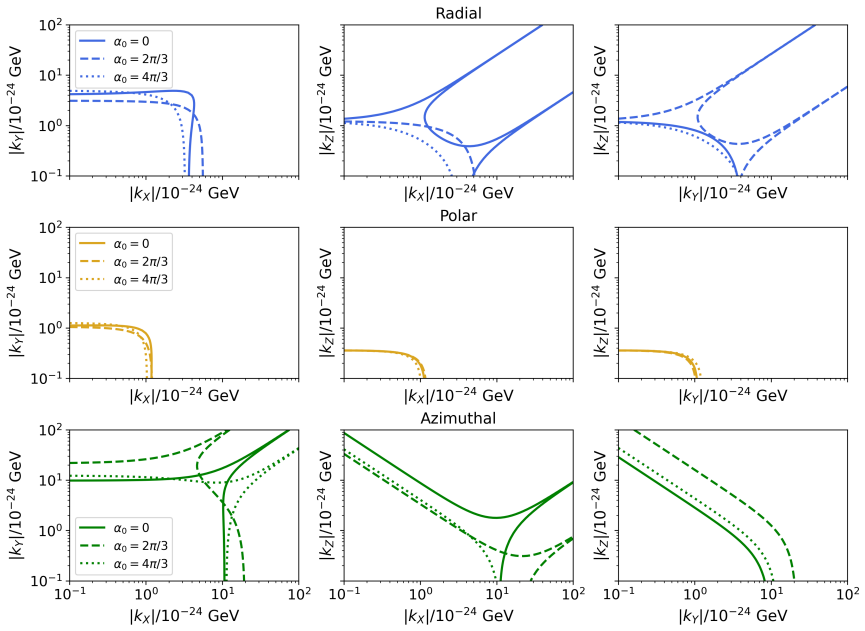
We solve the field equations using the Green's method for a static point-like magnetic dipole and find the k_AF-dependent corrections to the standard dipolar magnetic field that strongly dominates the near-Earth magnetic field. Given the very good agreement between current models and ground- and satellite-based geomagnetic data, our strongest constraints on the components of k_AF in the Sun-centered frame read |(k_AF)_Z| ≲ 4 × 10^{-25} GeV for |(k_AF)_X|, |(k_AF)_Y| ≲ 10^{-24} GeV at the two-sigma level. This represents an improvement of about four orders of magnitude over earlier bounds based on other geophysical phenomena.
What carries the argument
The Green's function solution to the inhomogeneous Maxwell equations modified by the Carroll-Field-Jackiw term, which adds linear corrections in the components of the constant 4-vector k_AF to the usual dipole magnetic field.
If this is right
- The Z-component of k_AF receives the strongest constraint from the data.
- The derived limits are stated in the Sun-centered frame standard for Lorentz-violation studies.
- The same dipole-correction method improves bounds by four orders of magnitude relative to earlier geophysical analyses.
- Continued agreement between models and data directly tightens the allowed range for k_AF.
Where Pith is reading between the lines
- The same Green's-function approach could be applied to the magnetic fields of other planets to search for the identical correction pattern.
- Detection of a non-zero k_AF would imply a fixed spacetime direction that influences electromagnetic fields everywhere, not only near Earth.
- Future magnetometer arrays with improved precision could either detect the predicted directional corrections or push the bounds lower still.
Load-bearing premise
Any difference between the observed geomagnetic field and the predictions of ordinary dipole models is assumed to arise solely from the Carroll-Field-Jackiw term rather than from unmodeled internal Earth processes, measurement errors, or imperfections in the baseline models.
What would settle it
A high-resolution global map of the geomagnetic field that exhibits systematic angular deviations matching the exact pattern predicted by a non-zero k_AF at or above the quoted bound, after subtraction of all known geophysical contributions, would support the term; tighter agreement with the uncorrected dipole would reinforce the limit.
Figures


read the original abstract
Lorentz-symmetry violation may be described via the CPT-odd, dimension-3, Carroll-Field-Jackiw term, which couples the electromagnetic fields to a constant 4-vector $k_{\rm AF}$ selecting a preferred direction in spacetime. We solve the field equations using the Green's method for a static point-like magnetic dipole and find the $k_{\rm AF}$-dependent corrections to the standard dipolar magnetic field that strongly dominates the near-Earth magnetic field. Given the very good agreement between current models and ground- and satellite-based geomagnetic data, our strongest constraints on the components of $k_{\rm AF}$ in the Sun-centered frame read $|(k_{\rm AF})_Z| \lesssim 4 \times 10^{-25} \, {\rm GeV}$ for $|(k_{\rm AF})_X|, |(k_{\rm AF})_Y| \lesssim 10^{-24} \, {\rm GeV}$ at the two-sigma level. This represents an improvement of about four orders of magnitude over earlier bounds based on other geophysical phenomena.
Editorial analysis
A structured set of objections, weighed in public.
Referee Report
Summary. The manuscript solves the modified static Maxwell equations including the Carroll-Field-Jackiw (CFJ) term for a point-like magnetic dipole using Green's functions. It obtains k_AF-dependent corrections to the standard dipole field and, citing the close agreement between current geomagnetic models and ground/satellite data, extracts two-sigma bounds |(k_AF)_Z| ≲ 4 × 10^{-25} GeV and |(k_AF)_X|, |(k_AF)_Y| ≲ 10^{-24} GeV in the Sun-centered frame, claiming a four-order-of-magnitude improvement over prior geophysical limits.
Significance. If the central mapping from data-model agreement to k_AF bounds is robust, the result would tighten existing constraints on the CPT-odd dimension-3 Lorentz-violating coefficient by four orders of magnitude using well-established geomagnetic datasets. The explicit Green's-function treatment of the modified dipole field is a technical strength that could be useful for other applications.
major comments (2)
- [Abstract and the section presenting the bounds] The extraction of the quoted bounds assumes that residuals between observed geomagnetic data and standard dipole models can be attributed entirely to the CFJ correction. The manuscript does not provide a quantitative error budget showing that contributions from higher multipoles, secular variation, ionospheric currents, or baseline-model systematics are smaller than the size of the k_AF-induced correction at the claimed 10^{-24}–10^{-25} GeV level.
- [Section deriving the Green's-function solution for the modified dipole field] The Green's-function solution is derived for a point-like static dipole. The manuscript does not address how the finite spatial extent of the Earth's core, mantle conductivity, or the distributed nature of the actual current sources modify the k_AF-dependent field corrections, which directly affects the reliability of the mapping to the reported limits.
minor comments (1)
- Clarify the precise definition and normalization of the Sun-centered frame components of k_AF with an explicit reference to the standard conventions used in the Lorentz-violation literature.
Simulated Author's Rebuttal
We thank the referee for the thorough review and valuable feedback on our manuscript. We address the major comments point by point below and outline the revisions we plan to make to strengthen the presentation of our results.
read point-by-point responses
-
Referee: [Abstract and the section presenting the bounds] The extraction of the quoted bounds assumes that residuals between observed geomagnetic data and standard dipole models can be attributed entirely to the CFJ correction. The manuscript does not provide a quantitative error budget showing that contributions from higher multipoles, secular variation, ionospheric currents, or baseline-model systematics are smaller than the size of the k_AF-induced correction at the claimed 10^{-24}–10^{-25} GeV level.
Authors: We agree that a more explicit discussion of systematic uncertainties would strengthen the manuscript. In the revised version we will insert a new paragraph following the presentation of the bounds. There we will quote published residual levels from standard geomagnetic models (typically a few nT for the dipole component at the surface, corresponding to fractional corrections well above our claimed k_AF sensitivity) and note that any unmodeled contribution at that level would produce an apparent k_AF larger than our limit if misinterpreted as Lorentz violation. Because the CFJ correction possesses a unique vectorial structure aligned with the Sun-centered frame, it is distinguishable in principle from isotropic or randomly distributed systematics. We will also state that our limits are conservative upper bounds derived from the observed level of agreement rather than from a direct attribution of all residuals to k_AF. A full global fit separating all contributions lies beyond the present scope but is identified as a natural extension. revision: yes
-
Referee: [Section deriving the Green's-function solution for the modified dipole field] The Green's-function solution is derived for a point-like static dipole. The manuscript does not address how the finite spatial extent of the Earth's core, mantle conductivity, or the distributed nature of the actual current sources modify the k_AF-dependent field corrections, which directly affects the reliability of the mapping to the reported limits.
Authors: The point-dipole source is the standard leading-order description of the geomagnetic field exterior to the Earth, and the Green's-function solution captures the leading k_AF correction to that field. For a distributed current distribution the total correction would be obtained by integrating the same Green's function over the source volume. Because the CFJ term modifies the differential operators uniformly, the relative size of the correction at satellite altitudes remains comparable to the point-source result provided the source region is small compared with the observation distance. We will add a clarifying paragraph in the revised manuscript that makes this superposition argument explicit, cites the core radius (~0.55 Earth radii) versus typical satellite altitudes, and notes that static conductivity screening does not alter the leading-order correction. A complete numerical integration over a realistic core model is computationally demanding and is left for future work; however, we expect it to affect only sub-leading numerical factors and not the order-of-magnitude bounds reported here. revision: partial
Circularity Check
Derivation chain is independent of inputs; bounds from external data agreement
full rationale
The paper solves the modified Maxwell equations with the CFJ term via Green's function for a static point dipole to obtain explicit k_AF-dependent corrections to the standard dipole field. These corrections are then compared against the observed agreement between geomagnetic data and standard models from external sources. No equation reduces to a self-definition, no fitted parameter is relabeled as a prediction, and no load-bearing premise relies on a self-citation chain. The result is a constraint derived from the size of allowable corrections being smaller than residuals in independent datasets.
Axiom & Free-Parameter Ledger
axioms (2)
- domain assumption The electromagnetic field equations are modified by the addition of the Carroll-Field-Jackiw term coupling F to a constant 4-vector k_AF.
- domain assumption The near-Earth magnetic field is accurately described by a static point-like magnetic dipole plus small corrections.
invented entities (1)
-
k_AF 4-vector
no independent evidence
Lean theorems connected to this paper
-
IndisputableMonolith/Foundation/AlexanderDuality.leanalexander_duality_circle_linking unclear?
unclearRelation between the paper passage and the cited Recognition theorem.
We solve the field equations using the Green's method for a static point-like magnetic dipole and find the k_AF-dependent corrections to the standard dipolar magnetic field... |(k_AF)_Z| ≲ 4 × 10^{-25} GeV
-
IndisputableMonolith/Cost/FunctionalEquation.leanwashburn_uniqueness_aczel unclear?
unclearRelation between the paper passage and the cited Recognition theorem.
The CFJ magnetic field... is composed of three pieces: the first is the Maxwellian dipolar field BM(x) = ... corrected by ... exclusively CFJ-originated contributions BCFJ(x)
What do these tags mean?
- matches
- The paper's claim is directly supported by a theorem in the formal canon.
- supports
- The theorem supports part of the paper's argument, but the paper may add assumptions or extra steps.
- extends
- The paper goes beyond the formal theorem; the theorem is a base layer rather than the whole result.
- uses
- The paper appears to rely on the theorem as machinery.
- contradicts
- The paper's claim conflicts with a theorem or certificate in the canon.
- unclear
- Pith found a possible connection, but the passage is too broad, indirect, or ambiguous to say the theorem truly supports the claim.
Reference graph
Works this paper leans on
- [1]
-
[2]
V. A. Kosteleck´ y and S. Samuel. Spontaneous Breaking of Lorentz Symmetry in String Theory.Phys. Rev. D, 39:683, 1989
work page 1989
-
[3]
D. Colladay and V. A. Kosteleck´ y. CPT violation and the standard model.Phys. Rev. D, 55:6760–6774, 1997
work page 1997
-
[4]
D. Colladay and V. A. Kosteleck´ y. Lorentz-violating extension of the standard model. Phys. Rev. D, 58(11), 1998
work page 1998
-
[5]
V. A. Kosteleck´ y and N. Russell. Data tables for Lorentz and CPT violation.Reviews of Modern Physics, 83(1):11–31, 2011
work page 2011
-
[6]
S. M. Carroll, G. B. Field, and R. Jackiw. Limits on a Lorentz and Parity Violating Modification of Electrodynamics.Phys. Rev. D, 41:1231, 1990
work page 1990
-
[7]
C. Adam and F.R. Klinkhamer. Causality and CPT violation from an Abelian Chern–Simons-like term.Nucl. Phys. B, 607(1–2):247–267, 2001
work page 2001
- [8]
-
[9]
M. Goldhaber and V. Trimble. Limits on the chirality of interstellar and intergalactic space.J. Astrophys. Astron., 17:17, 1996. 51
work page 1996
-
[10]
V. A. Kosteleck´ y and M. Mewes. Astrophysical Tests of Lorentz and CPT Violation with Photons.Astrophys. J. Lett., 689:L1–L4, 2008
work page 2008
-
[11]
L. Pogosian, M. Shimon, M. Mewes, and B. Keating. Future CMB constraints on cosmic birefringence and implications for fundamental physics.Phys. Rev. D, 100(2):023507, 2019
work page 2019
-
[12]
A. D. A. M. Spallicci, G. Sarracino, O. Randriamboarison, J. A. Helay¨ el-Neto, and A. Dib. Testing the Amp` ere–Maxwell law on the photon mass and Lorentz symmetry violation with MMS multi-spacecraft data.The European Physical Journal Plus, 139(6), 2024
work page 2024
-
[13]
M. Mewes. Bounds on Lorentz and CPT violation from the Earth-ionosphere cavity. Physical Review D, 78(9), 2008
work page 2008
-
[14]
F.S. Ribeiro, P.D.S. Silva, and M.M. Ferreira. Constraining CPT-odd electromagnetic chiral parameters with pulsar timing.Phys. Rev. D, 112(3), 2025
work page 2025
- [15]
-
[16]
V. A. Kosteleck´ y, N. Russell, and J. D. Tasson. Constraints on Torsion from Bounds on Lorentz Violation.Phys. Rev. Lett., 100:111102, 2008
work page 2008
-
[17]
V. A. Kostelecky and R. Potting. Gravity from local Lorentz violation.Gen. Rel. Grav., 37:1675–1679, 2005
work page 2005
-
[18]
Q. G. Bailey and V. A. Kostelecky. Signals for Lorentz violation in post-Newtonian gravity. Phys. Rev. D, 74:045001, 2006
work page 2006
-
[19]
Y. M. P. Gomes and P. C. Malta. Laboratory-based limits on the Carroll-Field-Jackiw Lorentz-violating electrodynamics.Phys. Rev. D, 94:025031, 2016
work page 2016
-
[20]
L. H. C. Borges and A. F. Ferrari. External sources in a minimal and nonminimal CPT-odd Lorentz violating Maxwell electrodynamics.Modern Physics Letters A, 37(04), 2022. 52
work page 2022
-
[21]
A.H. Gomes, J.M. Fonseca, W.A. Moura-Melo, and A.R. Pereira. Testing CPT- and Lorentz-odd electrodynamics with waveguides.Journal of High Energy Physics, 2010(5), 2010
work page 2010
- [22]
-
[23]
Y. Bai, S. Lu, and N. Orlofsky. Searching for Magnetic Monopoles with Earth’s Magnetic Field.Phys. Rev. Lett., 127(10), August 2021
work page 2021
-
[24]
L. Zheng-Ting, L. Jun-Xu, G. Li-Sheng, K. Wei, and W. Ji. Constraining the Fifth Force Using the Earth as a Spin and Mass Source from the Chinese Space Station. 2024
work page 2024
-
[25]
L.R. Hunter and D.G. Ang. Using Geoelectrons to Search for Velocity-Dependent Spin- Spin Interactions.Phys. Rev. Lett., 112(9), March 2014
work page 2014
-
[26]
N.B. Clayburn and L.R. Hunter. Using Earth to search for long-range spin-velocity inter- actions.Phys. Rev. D, 108(5), September 2023
work page 2023
-
[27]
A. Arza, M. A. Fedderke, P. W. Graham, D. F. Jackson Kimball, and S. Kalia. Earth as a transducer for axion dark-matter detection.Phys. Rev. D, 105(9), 2022
work page 2022
-
[28]
I.A. Sulai et al. Hunt for magnetic signatures of hidden-photon and axion dark matter in the wilderness.Phys. Rev. D, 108(9), 2023
work page 2023
-
[29]
M. A. Fedderke, P. W. Graham, D. F. Jackson Kimball, and S. Kalia. Earth as a transducer for dark-photon dark-matter detection.Phys. Rev. D, 104(7), October 2021
work page 2021
-
[30]
M. A. Fedderke, P. W. Graham, D. F. Jackson Kimball, and S. Kalia. Search for dark- photon dark matter in the SuperMAG geomagnetic field dataset.Phys. Rev. D, 104(9), November 2021
work page 2021
-
[31]
E. Schr¨ odinger. The General Unitary Theory of the Physical Fields.Proceedings of the Royal Irish Academy. Section A: Mathematical and Physical Sciences, 49:43–58, 1943. 53
work page 1943
-
[32]
E. Schr¨ odinger. The Earth’s and the Sun’s Permanent Magnetic Fields in the Unitary Field Theory.Proceedings of the Royal Irish Academy. Section A: Mathematical and Physical Sciences, 49:135–148, 1943
work page 1943
-
[33]
A. S. Goldhaber and Michael M. Nieto. New geomagnetic limit on the mass of the photon. Phys. Rev. Lett., 21:567–569, 1968
work page 1968
-
[34]
E. Fischbach, H. Kloor, R. A. Langel, A. T. Y. Liu, and M. Peredo. New geomagnetic limits on the photon mass and on long range forces coexisting with electromagnetism. Phys. Rev. Lett., 73:514–517, 1994
work page 1994
-
[35]
V. A. Kosteleck´ y and M. Mewes. Signals for Lorentz violation in electrodynamics.Physical Review D, 66(5), September 2002
work page 2002
-
[36]
R. Bluhm, V.A. Kosteleck´ y, C.D. Lane, and N. Russell. Probing Lorentz violation with space-based experiments.Phys. Rev. D, 68(12), 2003
work page 2003
-
[37]
A. P. Baeta Scarpelli, H. Belich, J. L. Boldo, and J. A. Helay¨ el-Neto. Aspects of causality and unitarity and comments on vortexlike configurations in an Abelian model with a Lorentz-breaking term.Physical Review D, 67(8), April 2003
work page 2003
-
[38]
John David Jackson.Classical electrodynamics. Wiley, New York, NY, 3rd ed. edition, 1999
work page 1999
-
[39]
D.J. Cross. Resolution of the Mansuripur Paradox. 2012
work page 2012
-
[40]
M. Landeau et al. Sustaining Earth’s magnetic dynamo.Nat. Rev. Earth Environ., 3:255–269, 2022
work page 2022
-
[41]
B.A. Buffett. Earth’s Core and the Geodynamo.Science, 288(5473):2007–2012, 2000
work page 2007
-
[42]
A. Fournier, G. Hulot, and D. ad others Jault. Data Assimilation and Predictability in Geomagnetism.Space Sci Rev, 155:247–291, 2010
work page 2010
-
[43]
D. E. Winch, D. J. Ivers, J. P. R. Turner, and R. J. Stening. Geomagnetism and Schmidt quasi-normalization.Geophysical Journal International, 160(2):487–504, 2005. 54
work page 2005
-
[44]
T. J. Sabaka, G. Hulot, and N. Olsen.Mathematical Properties Relevant to Geomagnetic Field Modeling. Springer, 2010
work page 2010
-
[45]
A. Chulliat et al. The US/UK World Magnetic Model for 2025-2030: Technical Report. National Centers for Environmental Information, NOAA, 2025
work page 2025
-
[46]
P. Alken et al. International Geomagnetic Reference Field: the thirteenth generation. Earth, Planets and Space, 2021
work page 2021
-
[47]
Campbell.Introduction to geomagnetic fields
W.H. Campbell.Introduction to geomagnetic fields. Cambridge University Press, 2003
work page 2003
-
[48]
K.M. Laundal and A.D. Richmond. Magnetic Coordinate Systems.Space Sci. Rev., 206:27– 59, 2017
work page 2017
-
[49]
E. Th´ ebault, G. Hulot, B. Langlais, and P. Vigneron. A Spherical Harmonic Model of Earth’s Lithospheric Magnetic Field up to Degree 1050.Geophysical Research Letters, 48(21):e2021GL095147, 2021
work page 2021
- [50]
- [51]
-
[52]
Y. Choi et al. World Digital Magnetic Anomaly Map version 2.2. For an interesting visualization, see:https://wdmam.org
-
[53]
V. Lesur et al. Building the second version of the World Digital Magnetic Anomaly Map (WDMAM).Earth Planet Sp, 68(27):e2021GL095147, 2016
work page 2016
-
[54]
S. Maus and H. Luehr. Signature of the quiet-time magnetospheric magnetic field and its electromagnetic induction in the rotating Earth.Geophysical Journal International, 162(3):755–763, 09 2005. 55
work page 2005
-
[55]
S. W. H. Cowley. The Earth’s magnetosphere: A brief beginner’s guide.Eos, Transactions American Geophysical Union, 76(51):525–529, 1995
work page 1995
-
[56]
Y. Yamazaki and A. Maute. Sq and EEJ—A Review on the Daily Variation of the Ge- omagnetic Field Caused by Ionospheric Dynamo Currents.Space Sci Rev, 206:299–405, 2017
work page 2017
- [57]
-
[58]
S.E. Millan et al. Overview of Solar Wind–Magnetosphere–Ionosphere–Atmosphere Cou- pling and the Generation of Magnetospheric Currents.Space Sci Rev, 206:547–573, 2017
work page 2017
-
[59]
T.J. Sabaka et al. CM6: a comprehensive geomagnetic field model derived from both CHAMP and Swarm satellite observations.Earth Planets Space, 72:80, 2020
work page 2020
-
[60]
N. Olsen. Accounting for quiet-time magnetospheric field contributions in geomagnetic field modelling.Physics of the Earth and Planetary Interiors, 366:107411, 2025
work page 2025
-
[61]
C.C. Finlay et al. The CHAOS-7 geomagnetic field model and observed changes in the South Atlantic Anomaly.Earth, Planets and Space, 72(1), 2020
work page 2020
-
[62]
R.A. Langel, T.J. Sabaka, R.T. Baldwin, and J.A. Conrad. The near-Earth magnetic field from magnetospheric and quiet-day ionospheric sources and how it is modeled.Physics of the Earth and Planetary Interiors, 98(3):235–267, 1996
work page 1996
-
[63]
M. Fillion, A. Chulliat, P. Alken, M. Kruglyakov, A. Kuvshinov, and Neesha Schnepf. A Model of Hourly Variations of the Near-Earth Magnetic Field Generated in the Inner Magnetosphere and Its Induced Counterpart.Journal of Geophysical Research: Space Physics, 128(12):e2023JA031913, 2023
work page 2023
-
[64]
P. Alken et al. Evaluation of candidate models for the 13th generation International Geomagnetic Reference Field.Earth Planets Space, 73(48), 2021. 56
work page 2021
-
[65]
E. Friis-Christensen, H. L¨ uhr, and G. Hulot. Swarm: a constellation to study the Earth’s magnetic field.Earth Planets Space, 58(4), 2006
work page 2006
-
[66]
Nils Olsen, Giuseppe Albini, Jerome Bouffard, Tommaso Parrinello, and Lars Tøffner- Clausen. Magnetic observations from cryosat-2: calibration and processing of satellite platform magnetometer data.Earth, Planets and Space, 72(1):48, April 2020
work page 2020
-
[67]
C.D. Beggan. Evidence-based uncertainty estimates for the International Geomagnetic Reference Field.Earth Planets Space, 74(17), 2022
work page 2022
-
[68]
INTERMAGNET, International Real-time Magnetic Observatory Network,https:// intermagnet.org
-
[69]
See here for details:https://wdc.bgs.ac.uk/data.html
- [70]
-
[71]
Y. Yamazaki, J. Matzka, C. Stolle, G. Kervalishvili, J. Rauberg, O. Bronkalla, A. Morschhauser, S. Bruinsma, Y. Y. Shprits, and D. R. Jackson. Geomagnetic Activity Index Hpo.Geophysical Research Letters, 49(10):e2022GL098860, 2022
work page 2022
- [72]
-
[73]
A. Chulliat, P. Vigneron, and G. Hulot. First results from the Swarm Dedicated Ionospheric Field Inversion chain.Earth Planet Sp, 68(104), 2016
work page 2016
- [74]
-
[75]
N. Olsen and C. Stolle. Satellite geomagnetism.Annual Review of Earth and Planetary Sciences, 40:441–465, 2012
work page 2012
- [76]
-
[77]
J. van den IJssel, J. Encarna¸ c˜ ao, E. Doornbos, and P. Visser. Precise science orbits for the Swarm satellite constellation.Advances in Space Research, (6):1042–1055, 2015
work page 2015
-
[78]
Brown.Elements of Spacecraft Design
C.D. Brown.Elements of Spacecraft Design. American Institute of Aeronautics and As- tronautics, Inc., 2002
work page 2002
-
[79]
N.H. Crisp et al. The benefits of very low earth orbit for earth observation missions. Progress in Aerospace Sciences, 117:100619, 2020. [80]https://www.ucs.org/resources/satellite-database#.XELwRFxKjIW
work page 2020
-
[80]
L. Davis, Jr., A. S. Goldhaber, and Michael M. Nieto. Limit on the photon mass deduced from Pioneer-10 observations of Jupiter’s magnetic field.Phys. Rev. Lett., 35:1402–1405, 1975
work page 1975
discussion (0)
Sign in with ORCID, Apple, or X to comment. Anyone can read and Pith papers without signing in.