A logarithmic phase singularity at the heart of Landau-Zener transitions
Pith reviewed 2026-07-01 04:55 UTC · model grok-4.3
The pith
The Landau-Zener amplitude a_LZ is produced by a logarithmic phase singularity from a contour integral around a simple pole.
A machine-rendered reading of the paper's core claim, the machinery that carries it, and where it could break.
Core claim
Three ingredients determine the expression a_LZ ≡ exp[−π/(2ε)] for the asymptotic probability amplitude in the Landau-Zener problem: a wave phase given by the product of a contour integral over a simple pole at the origin and 1/(2ε), an asymptotic path connecting ±1 that circumvents the pole in the upper half-plane, and a closing half-circle in the lower half-plane. The Cauchy theorem assigns the value iπ to this contour and thereby yields a_LZ. The analysis shows that a_LZ follows from a logarithmic phase singularity and accounts for the Markov approximation result.
What carries the argument
Contour integral over the simple pole at the origin in the complex plane, evaluated along the specified asymptotic path and closing semicircle to give iπ by Cauchy's theorem.
If this is right
- The value a_LZ follows directly from applying Cauchy's theorem to the closed contour around the pole.
- The Markov approximation reproduces a_LZ because it preserves the same phase singularity from the pole.
- The result depends on the specific choice of path that avoids the pole in the upper half-plane.
- The logarithmic nature of the phase singularity is central to obtaining the exponential form of the amplitude.
Where Pith is reading between the lines
- This framing may extend to other two-level systems with linear sweeps by identifying analogous poles.
- Similar contour arguments could simplify derivations of transition probabilities in time-dependent quantum mechanics.
- Experimental verification might involve checking if small deviations from the ideal path alter the amplitude in predictable ways.
Load-bearing premise
The phase of the wave is determined by the product of a contour integral over a simple pole at the origin and the inverse of twice the scaled chirp parameter ε, together with the specific choice of asymptotic path connecting ±1 that circumvents the pole in the upper half-plane.
What would settle it
A direct evaluation of the contour integral showing it does not equal iπ for the described path would disprove that this mechanism produces a_LZ.
Figures
read the original abstract
Three ingredients of the elementary Landau-Zener problem determine the familiar expression $a_{LZ}\equiv\exp\left[-\pi/(2\epsilon)\right]$ for the asymptotic value of the probability amplitude for remaining in the initial level: (i) A wave whose phase is determined by the product of a contour integral over a simple pole at the origin of the complex plane and the inverse of twice the scaled chirp parameter $\epsilon$. (ii) An asymptotic limit of the associated path connecting the points $\pm 1$ along the real axis and circumventing the pole in the upper half-plane, and (iii) a half-circle in the lower half plane enclosing together with the asymptotic path the pole. The Cauchy theorem immediately provides us with the value $\ii\pi$ of the asymptotic contour, and thus with $a_{LZ}$. Our analysis demonstrates not only that $a_{LZ}$ is the consequence of a logarithmic phase singularity but also explains why the Markov approximation also leads to $a_{LZ}$.
Editorial analysis
A structured set of objections, weighed in public.
Referee Report
Summary. The paper claims that the standard Landau-Zener transition amplitude a_LZ ≡ exp[−π/(2ε)] is a direct consequence of a logarithmic phase singularity at the origin in the complex plane. It identifies three ingredients: (i) a wave phase given by the product of a contour integral over a simple pole at the origin and 1/(2ε), (ii) an asymptotic path from −1 to +1 along the real axis that circumvents the pole in the upper half-plane, and (iii) a closing half-circle in the lower half-plane. Application of Cauchy's theorem then yields the contour value iπ and thus a_LZ. The analysis is also said to explain why the Markov approximation produces the same result.
Significance. If the mapping from the LZ Schrödinger equation to the posited contour-integral phase were rigorously established, the work would supply a compact complex-analytic account of the LZ probability and its relation to the Markov limit. The approach is parameter-free once the contour is fixed and invokes only standard residue calculus, which would be a strength. However, the significance is currently undercut by the absence of a derivation linking the phase expression to the time-dependent Hamiltonian.
major comments (2)
- [Abstract] Abstract and opening paragraphs: the central claim requires that the phase of the wavefunction equals (contour integral over the simple pole at the origin) × (1/(2ε)) with the specific upper-half-plane path. No step derives this phase expression from the time-dependent Schrödinger equation for the standard LZ Hamiltonian H(t) = (ε t) σ_z + σ_x; the contour and path appear chosen to recover the known a_LZ rather than obtained from the dynamics. This identification is load-bearing for the assertion that a_LZ 'is the consequence of a logarithmic phase singularity.'
- [Abstract] Abstract: the statement that the analysis 'explains why the Markov approximation also leads to a_LZ' is asserted but not demonstrated. The manuscript must show explicitly how the Markov limit corresponds to the same contour or residue calculation; without that step the explanatory claim remains unsupported.
minor comments (1)
- Notation: the scaled chirp parameter ε is introduced without an explicit definition relating it to the conventional LZ parameter; a one-line equation linking ε to the Hamiltonian coefficients would remove ambiguity.
Simulated Author's Rebuttal
We thank the referee for the careful reading and for identifying points where the presentation can be strengthened. We address each major comment below and will revise the manuscript accordingly.
read point-by-point responses
-
Referee: [Abstract] Abstract and opening paragraphs: the central claim requires that the phase of the wavefunction equals (contour integral over the simple pole at the origin) × (1/(2ε)) with the specific upper-half-plane path. No step derives this phase expression from the time-dependent Schrödinger equation for the standard LZ Hamiltonian H(t) = (ε t) σ_z + σ_x; the contour and path appear chosen to recover the known a_LZ rather than obtained from the dynamics. This identification is load-bearing for the assertion that a_LZ 'is the consequence of a logarithmic phase singularity.'
Authors: The referee is correct that the current manuscript introduces the phase expression as one of the three ingredients without an explicit step-by-step derivation from the time-dependent Schrödinger equation. The focus of the work is on the complex-analytic consequences once that phase form is accepted. In the revision we will add a dedicated paragraph (or short subsection) that motivates the phase from the semiclassical/WKB treatment of the LZ problem, showing how the contour and the upper-half-plane path follow from the asymptotic behavior of the wave function for the standard Hamiltonian. This will make the load-bearing identification explicit rather than implicit. revision: yes
-
Referee: [Abstract] Abstract: the statement that the analysis 'explains why the Markov approximation also leads to a_LZ' is asserted but not demonstrated. The manuscript must show explicitly how the Markov limit corresponds to the same contour or residue calculation; without that step the explanatory claim remains unsupported.
Authors: We agree that the explanatory link to the Markov approximation is stated in the abstract and introduction but is not worked out in detail. In the revised manuscript we will insert a short paragraph that maps the Markov limit onto the same contour integral, showing that the residue evaluation remains unchanged and thereby accounts for the identical value of a_LZ. This will convert the assertion into an explicit demonstration. revision: yes
Circularity Check
No circularity: derivation applies external Cauchy theorem to stated phase ingredients without reduction to fitted values or self-citation chains
full rationale
The paper presents three ingredients—including a phase given by a contour integral over a simple pole scaled by 1/(2ε) with a specified asymptotic path—and invokes the external Cauchy theorem to obtain iπ and thus the known a_LZ = exp[-π/(2ε)]. No equation in the provided text reduces a_LZ to a parameter fitted inside the paper, renames a prior result, or relies on a load-bearing self-citation whose content is unverified. The derivation is self-contained as an interpretive mapping from standard complex analysis onto the LZ problem; the phase form is listed as an ingredient of the problem rather than derived via internal fitting or self-referential definition.
Axiom & Free-Parameter Ledger
axioms (1)
- standard math Cauchy integral theorem: integral over closed contour equals 2πi times enclosed residue for analytic functions except at simple poles.
Reference graph
Works this paper leans on
-
[1]
Formulation of the problem The Landau-Zener problem involves in its most ele- mentary version thelinearcrossing of two energy levels with a time-independent coupling. The corresponding Schr¨ odinger equations for the two probability amplitudes a=a(t) andb=b(t) read i d dt a=−αta+ Ωb,(2) i d dt b=αtb+ Ωa.(3) Here, t, α and Ω denotes time, the chirp involvi...
-
[2]
Obviously, the initial and final times −t0 andt 0 correspond toτ= 1 andτ=−1
Asymptotic scaling Therefore, it is useful to introduce the dimensionless time τ≡ t −t0 (8) which maps the time interval −t0 ≤t≤t 0 onto 1≥τ≥ −1 . Obviously, the initial and final times −t0 andt 0 correspond toτ= 1 andτ=−1. Thus, Eqs. (2) and (3) take the form i˙a=−ϵτ 2 0 τ a−τ 0b(9) i˙b=ϵτ 2 0 τ b−τ 0a(10) for the two probability amplitudes a=a(τ;τ 0) an...
-
[3]
(9) and (10), we first integrate the terms proportional to τ and then consider the remaining dynamics due to the coupling
Interaction picture In order to solve Eqs. (9) and (10), we first integrate the terms proportional to τ and then consider the remaining dynamics due to the coupling. This procedure corresponds to a transformation into the interaction picture. For this purpose, we now make the ansatz a(τ;τ 0)≡e iϵτ 2 0 (τ 2−1)/2˜a(τ;τ0) (13) with the initial condition ˜a(1...
-
[4]
(22), and make the ansatz ˜a(τ;τ0)≡exp i 2ϵ Z S ds1 s = exp i 2ϵ lnS (24) where the path S in the complex plane is defined in such a way that the right-hand side of Eq
Probability amplitude represented by a path We start by generalizing, Eq. (22), and make the ansatz ˜a(τ;τ0)≡exp i 2ϵ Z S ds1 s = exp i 2ϵ lnS (24) where the path S in the complex plane is defined in such a way that the right-hand side of Eq. (24) is identical to the solution of the differential equation, Eq. (18), subjected to the initial conditions Eqs....
-
[5]
These formulae allow us in the next section to de- termine the asymptotic path Sa
Avoidance of the pole and normalization condition We now present approximate analytical expressions for the path S for large values of τ0 in two different domains of τ. These formulae allow us in the next section to de- termine the asymptotic path Sa. We start the discussion by considering the caseτ→1. By direct differentiation, we can verify that S(|τ|;τ...
-
[6]
(30), for S follows immediately from the differential equation, Eq
Stueckelberg oscillations in the path For positive values of τ, the approximate expression, Eq. (30), for S follows immediately from the differential equation, Eq. (29), by a straightforward perturbative expansion in powers of 1 /τ 2 0 . Unfortunately, such an approach does not work for negative values ofτ. Indeed, in this domain the analog of g(+) depend...
-
[7]
(33), of ˜ain terms of the phase θ and the amplitude |S| of S, together with the probability interpretation of |˜a|2 enforces the use of positive values of θ, only
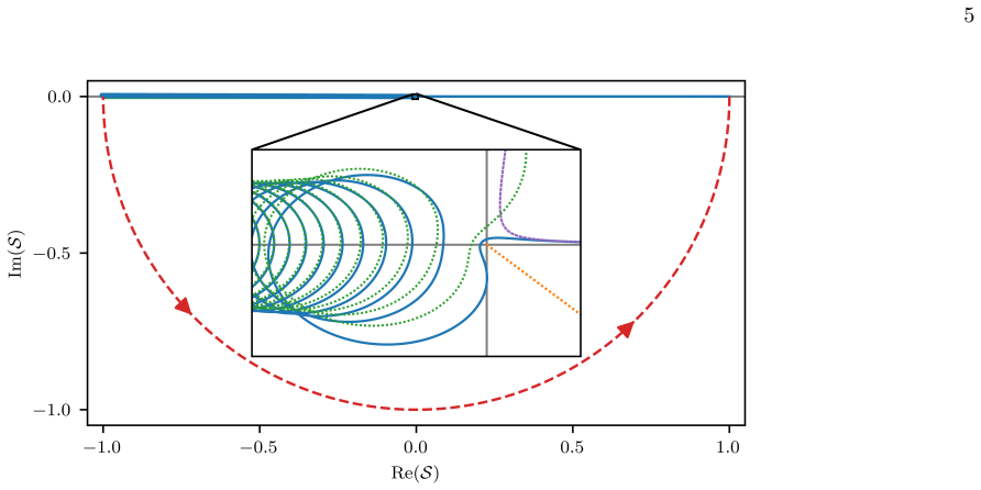
Choice of the branch cut The representation, Eq. (33), of ˜ain terms of the phase θ and the amplitude |S| of S, together with the probability interpretation of |˜a|2 enforces the use of positive values of θ, only. Moreover, Fig. 1 seems to suggest that the path S does not reach deep into the lower right quadrant, and in particular, circumvents the pole at...
-
[8]
2, we display the numerically obtained paths S for increasing values of τ0 and note that they move closer to the real axis
Asymptotic path and a subtlety In Fig. 2, we display the numerically obtained paths S for increasing values of τ0 and note that they move closer to the real axis. Moreover, the excursions to the upper half-plane as well as of the amplitudes of the oscillations for negative values ofτdecrease as well. In the limit of τ0 → ∞ , the resulting path connects th...
-
[9]
Indeed, for large but finite values of τ0, S(−1; τ0) is close to−1 but not identical to it, as shown by Fig
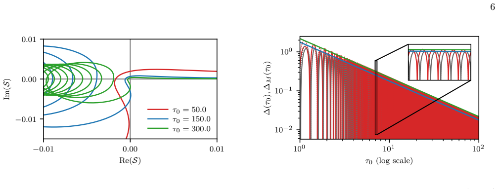
Approach of the endpoint of the path Moreover, we emphasize that the approach of the final point S(−1; τ0) of the path S towards −1 is non-uniform. Indeed, for large but finite values of τ0, S(−1; τ0) is close to−1 but not identical to it, as shown by Fig. 3. Here, we display the distance ∆(τ0)≡ |S(−1;τ 0) + 1|(39) ofS(−1;τ 0) from−1 for increasingτ 0. We...
-
[10]
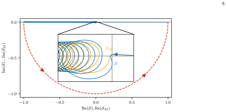
(29), the Markov path SM is given explicitly
Explicit expression In contrast to the exact path S which is defined by the differential equation, Eq. (29), the Markov path SM is given explicitly. Indeed, when we recall [ 38] the Markov solution ˜aM(τ;τ 0)≡e iHM (τ;τ 0) (42) with HM(τ;τ 0)≡iτ 2 0 Z τ 1 dτ ′e−iϵτ 2 0 τ ′2 Z τ ′ 1 dτ ′′eiϵτ 2 0 τ ′′2 ,(43) a comparison with Eq. (24) immediately provides ...
-
[11]
Avoidance of the pole This escape of SM also emerges analytically when we derive a differential equation for SM analogous to Eq. (29). Indeed, from Eqs. (43) and (44), we find by differentiation the nonlinear differential equation of second order 1 τ 2 0 i 2ϵ ¨SM SM − i 2ϵ ˙SM SM !2 −τ ˙SM SM + 1 = 0.(45) When we compare this equation for the Marko...
-
[12]
Stueckelberg oscillations in the Markov path In complete analogy to the exact path S, we derive in appendix A the approximate expression SM(−|τ|;τ 0) =−|τ| 1 + 1 τ0 g(−) M (−|τ|;τ 0) (48) for the Markov path valid for negative values of τ. Here, we have introduced the abbreviations g(−) M (−|τ|;τ 0)≡ r π ϵ 1 |τ| eiϵτ 2 0(τ 2−1)eiφM (τ0) −e −iφM (τ0) (49) ...
-
[13]
Approach of the endpoint of the Markov path We are now in the position to analyze the approach of the Markov pathS M to−1 as defined by the distance ∆M(τ0)≡ |S M(−1;τ 0) + 1|.(51) Indeed, when we substitute Eq. (48) into this expression we find ∆M(τ0) = 2 τ0 r π ϵ |sin [φM(τ0)]|.(52) Hence, the distance ∆ M from SM(−1; τ0) to −1 scales with 1 /τ0, in comp...
-
[14]
When we substitute the definition, Eq
Asymptotics of exact solution In the scaling of the present article, the expression for the probability amplitude a in the limit of negative values of τ, that is for positive timestreads a(−|τ|;τ 0) = f(−|τ|;τ 0) f(1;τ 0) 1 + i 2ϵ 1 τ0 g(−)(−|τ|;τ 0) (A1) where we have introduced the elementary wave f(τ;τ 0)≡e iϵτ 2 0 τ 2/2e i 2ϵ ln(τ τ0) (A2) 10 and the ...
-
[15]
r iπ ϵ + eiϵτ 2 0 iϵτ0 # (A17) and Z −|τ| 0 dτ ′e−iϵτ 2 0 τ ′2 ∼= − 1 2τ0
Markov approximation In the scaling of the present article, the Markov solution [38] reads aM(τ;τ 0)≡e iϵτ 2 0(τ 2−1)/2eiHM (τ;τ 0) (A10) with HM(τ;τ 0)≡iτ 2 0 Z τ 1 dτ ′e−iϵτ 2 0 τ ′2 Z τ ′ 1 dτ ′′eiϵτ 2 0 τ ′′2 ,(A11) and leads us to the expression SM(τ;τ 0) = e2ϵHM (τ;τ 0) (A12) for the Markov path. We recall from Ref. [38] the identity HM(−|τ|;τ 0) = ...
-
[16]
S. W. Hawking, Black hole explosions?, Nature248, 30 (1974)
1974
-
[17]
W. G. Unruh, Notes on black-hole evaporation, Phys. Rev. D14, 870 (1976)
1976
-
[18]
S. W. Hawking, The Quantum Mechanics of Black Holes, Scientific American236, 34 (1977)
1977
-
[19]
M. O. Scully, S. Fulling, D. M. Lee, D. N. Page, W. P. Schleich, and A. A. Svidzinsky, Quantum optics approach to radiation from atoms falling into a black hole, Pro- ceedings of the National Academy of Sciences115, 8131 (2018)
2018
-
[20]
Ullinger, M
F. Ullinger, M. Zimmermann, and W. P. Schleich, The logarithmic phase singularity in the inverted harmonic oscillator, AVS Quantum Science4, 024402 (2022)
2022
-
[21]
G. G. Rozenman, F. Ullinger, M. Zimmermann, M. A. Efremov, L. Shemer, W. P. Schleich, and A. Arie, Obser- vation of a phase space horizon with surface gravity water waves, Communications Physics7, 165 (2024)
2024
-
[22]
L. D. Landau, A theory of energy transfer. II, Collected Papers of L.D. Landau , 63 (1965)
1965
-
[23]
Zener, Non-adiabatic crossing of energy levels, Proc
C. Zener, Non-adiabatic crossing of energy levels, Proc. R. Soc. London A137, 696 (1932)
1932
-
[24]
Majorana, Atomi orientati in campo magnetico vari- abile, Il Nuovo Cimento9, 43 (1932)
E. Majorana, Atomi orientati in campo magnetico vari- abile, Il Nuovo Cimento9, 43 (1932). 12
1932
-
[25]
E. C. G. Stueckelberg, Theorie der unelastischen St¨ osse zwischen Atomen, Helvetica Physica Acta5, 369 (1932)
1932
-
[26]
A. M. Dykhne, Adiabatic perturbation of discrete spec- trum states, Sov. Phys. JETP11, 411 (1960), zh. Eksp. Teor. Fiz.38, 570 (1960)
1960
-
[27]
Suominen, B
K.-A. Suominen, B. Garraway, and S. Stenholm, The adiabatic limit of level crossing models, Optics Communi- cations82, 260 (1991)
1991
-
[28]
Suominen and B
K.-A. Suominen and B. M. Garraway, Population transfer in a level-crossing model with two time scales, Phys. Rev. A45, 374 (1992)
1992
-
[29]
V. M. Akulin and W. P. Schleich, Landau-Zener transition to a decaying level, Phys. Rev. A46, 4110 (1992)
1992
-
[30]
N. V. Vitanov, Transition times in the Landau-Zener model, Phys. Rev. A59, 988 (1999)
1999
-
[31]
J. Liu, L. Fu, B.-Y. Ou, S.-G. Chen, D.-I. Choi, B. Wu, and Q. Niu, Theory of nonlinear Landau-Zener tunneling, Phys. Rev. A66, 023404 (2002)
2002
-
[32]
Nakamura,Nonadiabatic Transition: Concepts, Basic Theories and Applications(World Scientific, 2012)
H. Nakamura,Nonadiabatic Transition: Concepts, Basic Theories and Applications(World Scientific, 2012)
2012
-
[33]
A. V. Shytov, Landau-Zener transitions in a multilevel system: An exact result, Phys. Rev. A70, 052708 (2004)
2004
-
[34]
E. Peik, M. Ben Dahan, I. Bouchoule, Y. Castin, and C. Salomon, Bloch oscillations of atoms, adiabatic rapid passage, and monokinetic atomic beams, Phys. Rev. A 55, 2989 (1997)
1997
-
[35]
Ankerhold and H
J. Ankerhold and H. Grabert, Enhancement of Macro- scopic Quantum Tunneling by Landau-Zener Transitions, Phys. Rev. Lett.91, 016803 (2003)
2003
-
[36]
Saito, M
K. Saito, M. Wubs, S. Kohler, Y. Kayanuma, and P. H¨ anggi, Dissipative Landau-Zener transitions of a qubit: Bath-specific and universal behavior, Phys. Rev. B75, 214308 (2007)
2007
-
[37]
K. A. Burrows, H. Perrin, and B. M. Garraway, Nona- diabatic losses from radio-frequency-dressed cold-atom traps: Beyond the Landau-Zener model, Phys. Rev. A96, 023429 (2017)
2017
-
[38]
Gebbe, J.-N
M. Gebbe, J.-N. Siemß, M. Gersemann, H. M¨ untinga, S. Herrmann, C. L¨ ammerzahl, H. Ahlers, N. Gaaloul, C. Schubert, K. Hammerer, S. Abend, and E. M. Rasel, Twin-lattice atom interferometry, Nature Communica- tions12, 2544 (2021)
2021
-
[39]
Fitzek, J.-N
F. Fitzek, J.-N. Kirsten-Siemß, E. M. Rasel, N. Gaaloul, and K. Hammerer, Accurate and efficient Bloch- oscillation-enhanced atom interferometry, Phys. Rev. Res. 6, L032028 (2024)
2024
-
[40]
P. O. Kofman, S. N. Shevchenko, and F. Nori, Tuning the initial phase to control the final state of a driven qubit, Phys. Rev. A109, 022409 (2024)
2024
-
[41]
Konrad and M
B. Konrad and M. Efremov, Angular Bloch oscillations and their applications, Quantum Science and Technology 10, 015025 (2024)
2024
-
[42]
Bj¨ orkman, M
I. Bj¨ orkman, M. Kuzmanovi´ c, and G. S. Paraoanu, Ob- servation of the Two-Photon Landau-Zener-St¨ uckelberg- Majorana Effect, Phys. Rev. Lett.134, 060602 (2025)
2025
-
[43]
D. O. Shendryk, O. V. Ivakhnenko, S. N. Shevchenko, and F. Nori, Efficient implementation of quantum signal processing via the adiabatic-impulse model, Phys. Rev. A 112, 042437 (2025)
2025
-
[44]
J. R. F. Lima and G. Burkard, Partial Landau-Zener transitions and applications to qubit shuttling, Phys. Rev. B111, 235439 (2025)
2025
-
[45]
M. V. Berry and R. Lim, Universal transition prefactors derived by superadiabatic renormalization, Journal of Physics A: Mathematical and General26, 4737 (1993)
1993
-
[46]
Kayanuma, Stokes phase and geometrical phase in a driven two-level system, Phys
Y. Kayanuma, Stokes phase and geometrical phase in a driven two-level system, Phys. Rev. A55, R2495 (1997)
1997
-
[47]
P. O. Kofman, O. V. Ivakhnenko, S. N. Shevchenko, and F. Nori, Majorana’s approach to nonadiabatic transitions validates the adiabatic-impulse approximation, Scientific Reports13, 5053 (2023)
2023
-
[48]
L. A. J. Guttieres, M. D. Petrovi´ c, and J. K. Freericks, Computational projects with the Landau–Zener problem in the quantum mechanics classroom, American Journal of Physics91, 885 (2023)
2023
-
[49]
Sun, Derivation of the Landau–Zener formula via func- tional equations, Journal of Physics A: Mathematical and Theoretical58, 37LT01 (2025)
C. Sun, Derivation of the Landau–Zener formula via func- tional equations, Journal of Physics A: Mathematical and Theoretical58, 37LT01 (2025)
2025
-
[50]
N. V. Vitanov and B. M. Garraway, Landau-Zener model: Effects of finite coupling duration, Phys. Rev. A53, 4288 (1996)
1996
-
[51]
Shevchenko, S
S. Shevchenko, S. Ashhab, and F. Nori, Lan- dau–Zener–St¨ uckelberg interferometry, Physics Reports 492, 1 (2010)
2010
-
[52]
B. T. Torosov and N. V. Vitanov, Pseudo-Hermitian Landau-Zener-St¨ uckelberg-Majorana model, Phys. Rev. A96, 013845 (2017)
2017
-
[53]
E. P. Glasbrenner, Y. Gerdes, S. Varr´ o, and W. P. Schleich, Riccati equation perspective on Landau-Zener transitions, Phys. Rev. Res.7, 043208 (2025)
2025
-
[54]
E. P. Glasbrenner and W. P. Schleich, Elementary asymp- totic approach to the Landau-Zener problem (2026), manuscript submitted for publication
2026
-
[55]
E. P. Glasbrenner and W. P. Schleich, The Landau–Zener formula made simple, Journal of Physics B: Atomic, Molec- ular and Optical Physics56, 104001 (2023)
2023
-
[56]
E. P. Glasbrenner, Y. Gerdes, S. Varr´ o, and W. P. Schleich, A different perspective on the Landau-Zener dynamics, inProceedings of the Second International Workshop on Quantum Nonstationary Systems, edited by A. Dodonov and C. C. H. Ribeiro (LF Editorial, 2024) 1st ed., Chap. 17, pp. 273–297
2024
-
[57]
A. M. Dykhne, Transition probability for nonstationary problems, Sov. Phys. JETP14, 941 (1962), zh. Eksp. Teor. Fiz.41, 1324 (1961)
1962
-
[58]
J. P. Davis and P. Pechukas, Nonadiabatic transitions induced by a time-dependent Hamiltonian in the semi- classical/adiabatic limit: The two-state case, The Journal of Chemical Physics64, 3129 (1976)
1976
-
[59]
Teranishi and H
Y. Teranishi and H. Nakamura, Semiclassical theory of time-dependent curve crossing problems, The Journal of Chemical Physics107, 1904 (1997)
1904
-
[60]
Enomoto and T
S. Enomoto and T. Matsuda, The exact WKB and the Landau-Zener transition for asymmetry in cosmological particle production, Journal of High Energy Physics2022, 131 (2022)
2022
-
[61]
O. V. Ivakhnenko, S. N. Shevchenko, and F. Nori, Nonadi- abatic Landau–Zener–St¨ uckelberg–Majorana transitions, dynamics, and interference, Physics Reports995, 1 (2023)
2023
-
[62]
M. O. Scully and M. S. Zubairy,Quantum Optics(Cam- bridge University Press, 1997)
1997
-
[63]
Paulisch, H
V. Paulisch, H. Rui, H. K. Ng, and B.-G. Englert, Beyond adiabatic elimination: A hierarchy of approximations for multi-photon processes, The European Physical Journal Plus129, 12 (2014)
2014
-
[64]
A. G. Rojo, Matrix exponential solution of the Landau- Zener problem (2010), arXiv:1004.2914 [quant-ph]. 13
work page internal anchor Pith review Pith/arXiv arXiv 2010
-
[65]
Zhu and H
C. Zhu and H. Nakamura, Stokes constants for a cer- tain class of second-order ordinary differential equations, Journal of Mathematical Physics33, 2697 (1992)
1992
discussion (0)
Sign in with ORCID, Apple, or X to comment. Anyone can read and Pith papers without signing in.