REVIEW 4 major objections 4 minor 23 references
On the Mechanisms of Weak-to-Strong Generalization: A Theoretical Perspective
T0 review · 4 major / 4 minor · reviewed 2026-08-07 · deepseek-v4-flash
Pith's one-line read A student trained on a weaker teacher's labels can beat that teacher through three provable mechanisms: compensating teacher under-regularization, using a task-aligned regularization penalty, and combining teacher-taught easy features…
desk verdict Ridge and weighted-ridge results are solid and worth refereeing; the nonlinear third mechanism is unproven and Proposition 10 is false as stated. read the letter →
The pith
A machine-rendered reading of the paper's core claim, the machinery that carries it, and where it could break.
The reading
What carries the argument
The machinery is high-dimensional random matrix theory. All error formulas are written in terms of the Stieltjes transform $m(\lambda;\gamma)$ of the Marchenko-Pastur law with $m_{p,1} = m(\lambda_p,\gamma_p)$ and $m_{p,2} = -\partial m/\partial\lambda$; the ridge proofs evaluate traces of products of resolvent matrices through asymptotic freeness, and the weighted-ridge proof uses the Sherman-Morrison formula to expand $(\tilde{\Sigma} + \lambda_s \Gamma^{-1})^{-1}$ when $\Gamma = I + d_X \hat{\beta}\hat{\beta}^\top$. For the nonlinear section, the load-bearing object is the information exponent $\kappa_\sigma$, the first non-zero Hermite coefficient of the link function, which makes direction $\beta_e$ easy and $\beta_h$ hard for the teacher; the proof that one gradient step preserves the student's spike relies on a Hermite expansion of the nonlinear feature map together with the spike scaling $\tau = o(\sqrt{d_X})$.
What would settle it
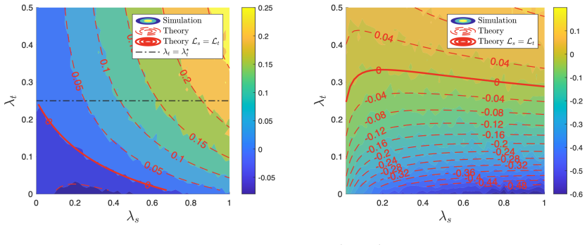
In the Section 2.1 setting, fix $\gamma_t$, $\gamma_s$, $\sigma^2_\varepsilon$ and choose teacher regularization $\lambda_t$ strictly above $\sigma^2_\varepsilon \gamma_t$; Theorem 5 predicts the student's limiting test error is never below the teacher's, so any simulation where some $\lambda_s$ yields $L_s < L_t$ would refute the ridge mechanism. For the nonlinear mechanism, initialize the student with $\tau = 0$ (no spike) and run one gradient step; the proof predicts no non-vanishing alignment to $\beta_h$, so observing non-trivial retention of $\beta_h$ without the spike would indicate a different mechanism is at work.
Extended reading notes
Core claim
The central discovery is a set of exact high-dimensional characterizations. For ridge regression with Gaussian features, the limiting test-error gap $L_s - L_t$ reduces to the closed form $\Delta = (\sigma^2_\varepsilon \gamma_t - \lambda_t)(m_{t,1} - \lambda_t m_{t,2})(\lambda_s^2 m_{s,2} - 2\lambda_s m_{s,1}) + \lambda_s^2 m_{s,2}(1 - \lambda_t m_{t,1})$, from which the paper proves that $L_s < L_t$ only when the teacher is under-regularized ($\lambda_t < \sigma^2_\varepsilon \gamma_t$) and the student's ridge parameter lies in a regime set by whether the student is under- or over-parameterized. For weighted ridge, the same gap becomes $\Delta - \zeta^2 \Delta_\Gamma$ with $\Delta_\Gamma \geq 0$, so enough alignment $\zeta$ between the student's regularization metric and the target lets the student win even at $\lambda_t = \lambda_t^*$. For two-layer networks, the proof shows that after one gradient step the student's first layer has non-vanishing operator norm along both the easy direction $\beta_e$ learned from the teacher and the hard direction $\beta_h$ inherited from its spiked pretrained initialization.
Load-bearing premise
The nonlinear result rests on the assumption that pretraining leaves the student's first layer with a rank-one spike aligned to the hard direction $\beta_h$; if real pretraining does not produce that clean low-rank spike, the third mechanism does not follow from the proof.
Editorial extensions
If this is right
- If the teacher is over-regularized ($\lambda_t \geq \sigma^2_\varepsilon \gamma_t$), no student ridge parameter produces weak-to-strong generalization in the linear setting; the student's only ridge route is to compensate under-regularization.
- The student's parameterization regime changes the recipe: an under-parameterized student ($\gamma_s < 1$) wins with any sufficiently small $\lambda_s$, while an over-parameterized student ($\gamma_s > 1$) wins only for $\lambda_s$ in an interval and only when condition (5) holds.
- A student with a regularization structure aligned to the target (positive $\zeta$ in Assumption 7) can beat even an optimally regularized teacher, and the benefit $-\zeta^2 \Delta_\Gamma$ grows with alignment.
- In the nonlinear model, a single gradient-descent step on teacher-generated labels is enough for the student to acquire the easy feature while keeping the hard feature, making early stopping provably sufficient rather than merely practical.
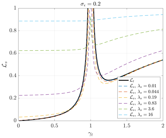
- The student's test error in this setting shows double descent as a function of the teacher's aspect ratio $\gamma_t$, and this double descent disappears when the teacher is optimally regularized.
Reading between the lines
- If the ridge characterization transfers to real fine-tuning, the practical lesson is to tune the student's regularization against the teacher's expected under-regularization: a teacher trained with too little regularization is exactly the regime where the student can gain.
- The weighted-ridge result suggests pretraining helps weak-to-strong generalization mainly by shaping the geometry of the student's penalty rather than just providing a better initialization; an experiment that varies feature alignment while controlling initialization could isolate this effect.
- The nonlinear proof only guarantees one gradient step; a natural testable extension is whether additional steps on teacher labels gradually erase the hard-feature spike, predicting an optimal fine-tuning length that the single-step theorem does not address.
- The three mechanisms are complementary rather than exhaustive; they suggest that diagnosing which mechanism applies in a given model may matter more than asking whether weak-to-strong occurs at all.
Editorial analysis
A structured set of objections, weighed in public.
Referee Report
Summary. The paper studies weak-to-strong generalization theoretically in three settings. In Setting 1, teacher and student are both high-dimensional ridge regressors and the paper derives an asymptotic formula for the test-error gap Ls - Lt and uses it to characterize when a student can beat an under-regularized teacher. In Setting 2, the student uses weighted ridge regularization whose structure is aligned with the target, and the paper derives a modified gap formula showing an additional favorable term. In Section 3, the paper analyzes one step of gradient descent in two-layer neural networks and claims a third mechanism: a pretrained student can acquire an easy, task-specific feature from the teacher while retaining a hard, transferable feature from pretraining. The linear results are supported by numerical simulations; the nonlinear results are not connected to any test-error comparison.
Significance. If the linear results are correct, the paper gives a useful and fairly complete asymptotic account of how teacher and student ridge regularization interact, a topic on which prior weak-to-strong theory has focused mostly on ridgeless regression or frozen representations. The explicit formulas in Theorems 4 and 8 are concrete, match the simulations shown, and lead to testable phase-transition predictions. The weighted-ridge mechanism is a reasonable formalization of the intuition that a student with better task-aligned structure can beat an optimally regularized teacher. The nonlinear section, by contrast, currently does not establish the third mechanism named in the abstract: it proves only first-layer alignment under a correlation loss, not superiority in test error, and the alignment statements themselves have gaps. The paper is therefore best viewed as a solid two-mechanism paper plus an underdeveloped third mechanism; that balance should be addressed explicitly in revision.
major comments (4)
- [Section 3, Proposition 10] The statement that ||hat(W)_t beta_h||_2 ->P 0 cannot follow from the proof. The proof shows only that the gradient projection ||nabla_{W_t} hat(L)_t beta_h||_2 ->P 0, whereas hat(W)_t = W_{t,0} - eta_t nabla_{W_t} hat(L)_t, so the updated vector contains W_{t,0} beta_h. With entries of W_{t,0} iid N(0,1/d_X) and p_t = Theta(d_X), ||W_{t,0} beta_h||_2 is Theta_P(1), not o_P(1). The same initialization issue affects the easy-direction claim: ||hat(W)_t beta_e||_2 has a Theta_P(1) random contribution from W_{t,0}, so a deterministic limit 'c > 0' is not established by the gradient calculation alone. Thus the teacher's failure to learn the hard direction is not proven in the sense claimed.
- [Section 3, Theorem 11 and 'Mechanism of Weak-to-Strong Generalization'] Theorem 11 proves only non-vanishing alignment of the student's first-layer weights to beta_e and beta_h, measured through the correlation loss in Eq. (10). No test error E_x[(f_s(x)-y)^2] is defined or bounded for the nonlinear models, and no comparison L_s < L_t is made. Moreover, the conclusion ||hat(W)_s beta_h||_op ->P c_h > 0 does not demonstrate retention of a pretrained spike: for W_{s,0} with iid N(0,1/d_X) entries and p_s = Theta(d_X), ||W_{s,0} beta_h||_2 is already Theta_P(1) for any unit beta_h, so c_h > 0 is satisfied at initialization even without the assumed spike. Since tau = o(sqrt(d_X)), the spike contribution is not guaranteed to dominate this random baseline. The abstract's third mechanism, that the student can outperform the teacher, is therefore not established by the stated results.
- [Section 2.1, Theorem 5 and Appendix D] Condition (5) in the main text is inconsistent with the appendix's condition (13). Appendix D derives two roots for gamma_s > 1 when c = (sigma_epsilon^2 gamma_t - lambda_t)/sqrt(-4 gamma_t + (1 + gamma_t + lambda_t)^2) satisfies c < 1/(1 - 4 gamma_s + sqrt(gamma_s(gamma_s - 1))); Equation (5) is a different, negated inequality with denominator 1 - 4 gamma_s - 4 sqrt(gamma_s^2 - gamma_s). The theorem's phase boundaries therefore do not follow from the proof as written. In addition, the proof concludes 'we have Delta < 1' where the required conclusion is Delta < 0, and the assertion that L_s >= L_t when (5) fails requires a sign argument that the root analysis alone does not provide.
- [Section 2.2, Theorem 8] The statement 'Additionally, we have Delta_Gamma >= 0' is made without proof. This sign claim is load-bearing: the conclusion that the term -zeta^2 Delta_Gamma always helps the student, including in the optimally-regularized-teacher regime in Figure 3, depends on it. A short derivation from the properties of m(lambda; gamma) would suffice, but as written the sign assertion is unsupported and should be proved or removed.
minor comments (4)
- [Section 3, Theorem 11 and its proof] The quantity ||hat(W)_s beta_h||_op should be the Euclidean norm of the vector hat(W)_s beta_h, not an operator norm; the proof also says 'Taking derivatives with respect to the matrix W_t' after defining the student loss, which should read W_s.
- [Assumption 7] The scaling remark '||I||_Fr asymptotically equivalent to ||d_X hat(beta) hat(beta)^T||_Fr' should refer to ||I_{d_X}||_Fr; as written, ||I||_Fr is ambiguous.
- [Figures 1 and 2 captions] The captions refer to dashed red contours, a solid curve, and a dashed black curve in a way that is easy to confuse; please harmonize the line-style and color references with the actual figures.
- [Section E and Appendix F] There are several typos, including 'fucntio' for 'function', 'ouperform' for 'outperform', 'lager' for 'larger', and 'scaler' for 'scalar'; a careful proofread is needed.
Circularity Check
No significant circularity: all three mechanisms are derived from explicit assumptions; the nonlinear section's conditional nature is a modeling choice, not a hidden reuse of the target result.
full rationale
The ridge-regression analysis (Section 2.1) and weighted-ridge analysis (Section 2.2) are self-contained asymptotic calculations: they start from Gaussian design assumptions, Marchenko-Pastur limits, and asymptotic freeness, and derive the test-error difference Ls−Lt (Theorems 4 and 8) without fitting any parameter to the target outcome. The optimal-teacher threshold λ⋆=σ²εγt is imported from an external result (Dobriban and Wager, 2018), and the weighted-ridge benefit is controlled by the explicitly assumed alignment ζ of Assumption 7, which is a free input of the theorem rather than a quantity reverse-engineered from Ls−Lt. Section 3 is explicitly conditional: Assumption 9 and the pretraining spike Ws,0=Wbar_s,0+τ abar β_hᵀ are stated, and Theorem 11 proves that this spike survives one gradient step while the student acquires the easy direction βe. That the student 'retains' the hard feature depends on the assumed spike, but the paper says so openly and the survival argument (G2=o(1)) is a derived property of the gradient, not an identity. The self-citations (Moniri et al. 2024; Moniri and Hassani 2024) are used as technical lemmas for Hermite expansions of nonlinear spiked random matrices; they are parameter-free published results and do not smuggle in the weak-to-strong conclusion. Separate correctness concerns exist—Proposition 10's proof shows only that the gradient's projection onto βh vanishes, whereas the random initialization contributes Θ_P(1) to ||Ŵtβh||, and Theorem 11 measures weight alignment rather than squared test error—but these are mathematical or evidential gaps, not circularity.
Assumptions & free parameters
free parameters (1)
- zeta (feature alignment in weighted ridge) =
set to 0.8, 0.88, 0.68, 0.89, 0.98 in simulations
assumptions (5)
- domain assumption Covariates are Gaussian: x_i ~ N(0, I_d) and target beta_star ~ N(0, d^{-1} I).
- standard math Asymptotic freeness of independent Wishart matrices (Voiculescu 1991), used to factor traces like Tr(hat_R^2 tilde_R^2).
- domain assumption Gamma has a rank-one spike: Gamma = I + d_X * betahat * betahat^T with correlation zeta.
- ad hoc to paper The student's pretrained weights already contain the hard direction: W_s,0 = Wbar_s,0 + tau * abar * beta_h^T with tau = o(sqrt(d_X)).
- domain assumption Information exponents: kappa_sigma_e = 1 and kappa_sigma_h > 1.
Cite this review
Pith. "Pith review of On the Mechanisms of Weak-to-Strong Generalization: A Theoretical Perspective." pith.science (2026). https://pith.science/paper/2XCUHGJE
@misc{pith2026250518346,
  author       = {Pith},
  title        = {Pith review of: On the Mechanisms of Weak-to-Strong Generalization: A Theoretical Perspective},
  year         = {2026},
  howpublished = {\url{https://pith.science/paper/2XCUHGJE}},
  note         = {Machine review of arXiv:2505.18346}
}
read the original abstract
Weak-to-strong generalization, where a student model trained on imperfect labels generated by a weaker teacher nonetheless surpasses that teacher, has been widely observed but the mechanisms that enable it have remained poorly understood. In this paper, through a theoretical analysis of simple models, we uncover three core mechanisms that can drive this phenomenon. First, by analyzing ridge regression, we study the interplay between the teacher and student regularization and prove that a student can compensate for a teacher's under-regularization and achieve lower test error. We also analyze the role of the parameterization regime of the models. Second, by analyzing weighted ridge regression, we show that a student model with a regularization structure more aligned to the target, can outperform its teacher. Third, in a nonlinear multi-index setting, we demonstrate that a student can learn easy, task-specific features from the teacher while leveraging its own broader pre-training to learn hard-to-learn features that the teacher cannot capture.
Figures


Figures from the paper (6 more)




Reference graph
Works this paper leans on
-
[1]
The solutions are given by ( λ− s , λ+ s ) from (12)
, two solutions exists for λs that satisfy for H1 = H2. The solutions are given by ( λ− s , λ+ s ) from (12). Consequently, we have ∆ < 1 as long as λs ∈ (λ− s , λ+ s ). These together finish the proof. E Non-Monotone Student Test Error Curves In this section, we study the the test error Ls as a function of γs and show that the student model also exhibits...
work page 2019
-
[2]
20 • Term 3, 4, 5, and 6: To analyze d −1 X Tr h ˆR2 ˜R2 i , we can use the asymptotic freeness of independent Wishart random matrices [Voiculescu, 1991] (see also Capitaine and Donati-Martin [2007]), and the Stone-Weierstrass theorem to approximate the function f (x) = (x + s)−2 using polynomials, to write d−1 X Tr h ˆR2 ˜R2 i = d−1 X Tr h ˆR2 i d−1 X Tr...
work page 1991
-
[3]
Learning two-layer neural networks, one (giant) step at a time
Yatin Dandi, Florent Krzakala, Bruno Loureiro, Luca Pesce, and Ludovic Stephan. Learning two-layer neural networks, one (giant) step at a time. arXiv preprint arXiv:2305.18270 ,
-
[4]
Samet Demir and Zafer Do˘ gan. Random features outperform linear models: Effect of strong input-label correlation in spiked covariance data. arXiv preprint arXiv:2409.20250 ,
-
[6]
Vision super- alignment: Weak-to-strong generalization for vision foundation models
Jianyuan Guo, Hanting Chen, Chengcheng Wang, Kai Han, Chang Xu, and Yunhe Wang. Vision super- alignment: Weak-to-strong generalization for vision foundation models. arXiv preprint arXiv:2402.03749 ,
-
[7]
Generalization for Least Squares Regression With Simple Spiked Covariances
Jiping Li and Rishi Sonthalia. Generalization for least squares regression with simple spiked covariances. arXiv preprint arXiv:2410.13991 ,
-
[8]
Co-supervised learning: Improving weak-to-strong generalization with hierarchical mixture of experts
14 Yuejiang Liu and Alexandre Alahi. Co-supervised learning: Improving weak-to-strong generalization with hierarchical mixture of experts. arXiv preprint arXiv:2402.15505 ,
-
[10]
Signal-plus-noise decomposition of nonlinear spiked random matrix models
Behrad Moniri and Hamed Hassani. Signal-plus-noise decomposition of nonlinear spiked random matrix models. arXiv preprint arXiv:2405.18274 ,
Show all 23 references
-
[11]
Relating misfit to gain in weak-to-strong generalization beyond the squared loss
Abhijeet Mulgund and Chirag Pabbaraju. Relating misfit to gain in weak-to-strong generalization beyond the squared loss. arXiv preprint arXiv:2501.19105 ,
-
[15]
Weak-to-strong reasoning
Yuqing Yang, Yan Ma, and Pengfei Liu. Weak-to-strong reasoning. In Findings of the Association for Computational Linguistics: EMNLP 2024 ,
2024
-
[17]
Note that using [Abramowitz and Stegun, 1968, Equation 22.8.8] we have d dx Hk(x) = kHk−1(x)
For any k ∈ N and x, y∈ R, we have Hk(x + y) = kX j=0 k j xjHk−j(y) Proof. Note that using [Abramowitz and Stegun, 1968, Equation 22.8.8] we have d dx Hk(x) = kHk−1(x). Thus, the j-th derivative of Hk is given by dj dxj Hk(x) = k! (k − j)! Hk−j(x). By Taylor expanding Hk(x + y...
1968
-
[20]
Figure 7: The test error of the student model Ls as a function of γt for σε = 1, γs = 0.1, λt → 0 (ridgeless), and different values of λs
24 Figure 6: The test error of the student model Ls as a function of γt for σε = 0.2, γs = 0.1, λt → 0 (ridgeless), and different values of λs. Figure 7: The test error of the student model Ls as a function of γt for σε = 1, γs = 0.1, λt → 0 (ridgeless), and different values o...
2021
-
[21]
From the definition of ms,1 and ms,2 and using the Marchenko-Pastur theorem, we have ˆβ⊤ ˜R2 ˆβ →P ms,2, and also ˆβ⊤ ˜R ˆβ →P ms,1
• For the third term, we can write ∥t3∥2 2 = ( ˆβ⊤ ˜R2 ˆβ) · λs 1 − λs ˆβ⊤ ˜R ˆβ 2 · ˆβ⊤ ˜R ˜Σ ˆR ˆΣβ⋆ 2 . From the definition of ms,1 and ms,2 and using the Marchenko-Pastur theorem, we have ˆβ⊤ ˜R2 ˆβ →P ms,2, and also ˆβ⊤ ˜R ˆβ →P ms,1. Also, we can write ˆβ⊤ ˜R ˜Σ ˆR ˆΣβ⋆ ...
1991
-
[22]
Thus, using [Vershynin, 2012, Theorem 5.44], we have ∥σ′ ⊥(Wt,0X⊤)∥op = O(√nt)
Thus, we can write ∇Wt bLt = − 1 nt h at y⊤ ⊙ cσ,1 + σ′ ⊥(Wt,0X⊤) i X = − cσ,1 nt at y⊤X − 1 nt h at y⊤ ⊙ σ′ ⊥(Wt,0X⊤) i X By construction, the matrix σ′ ⊥(Wt,0X⊤) has mean zero entries. Thus, using [Vershynin, 2012, Theorem 5.44], we have ∥σ′ ⊥(Wt,0X⊤)∥op = O(√nt). Hence, usi...
2012
-
[23]
as ˜y⊤ ⊙
This shows that the gradient has no alignment to the hard direction, completing the proof. 30 H Proof of Theorem 11 From the proof of Proposition 10, we have cWt = Wt,0 + cσ,1ηtat ˆβ⊤ e + ∆, where ˆβe = n−1 t X⊤y and ∥∆∥op = o(1). Given the fresh indepednent set of samples ˜X,...
2024
-
[1967]
Weak-to-strong generalization even in random feature networks, provably
Marko Medvedev, Kaifeng Lyu, Dingli Yu, Sanjeev Arora, Zhiyuan Li, and Nathan Srebro. Weak-to-strong generalization even in random feature networks, provably. arXiv preprint arXiv:2503.02877 ,
-
[1991]
Spectral evolution and invariance in linear-width neural networks
Zhichao Wang, Andrew Engel, Anand Sarwate, Ioana Dumitriu, and Tony Chiang. Spectral evolution and invariance in linear-width neural networks. arXiv preprint arXiv:2211.06506 ,
-
[2013]
Theorem 13 (Hanson-Wright Inequality [Hanson and Wright, 1971])
for a modern proof. Theorem 13 (Hanson-Wright Inequality [Hanson and Wright, 1971]). Let x = (X1, . . . , Xn) ∈ Rd be a random vector with independent sub-gaussian components Xi with EXi =
1971
-
[2021]
Your weak LLM is secretly a strong teacher for alignment
Leitian Tao and Yixuan Li. Your weak LLM is secretly a strong teacher for alignment. arXiv preprint arXiv:2409.08813,
-
[2022]
Provable weak-to-strong generalization via benign overfitting
David Xing Wu and Anant Sahai. Provable weak-to-strong generalization via benign overfitting. In NeurIPS 2024 Workshop on Mathematics of Modern Machine Learning ,
2024
-
[2023]
Repetita iuvant: Data repetition allows SGD to learn high-dimensional multi-index functions
12 Luca Arnaboldi, Yatin Dandi, Florent Krzakala, Luca Pesce, and Ludovic Stephan. Repetita iuvant: Data repetition allows SGD to learn high-dimensional multi-index functions. arXiv preprint arXiv:2405.15459 ,
-
[2024]
Risk and cross validation in ridge regression with correlated samples
Alexander Atanasov, Jacob A Zavatone-Veth, and Cengiz Pehlevan. Risk and cross validation in ridge regression with correlated samples. arXiv preprint arXiv:2408.04607 ,
-
[2025]
Spectral phase transitions in non-linear wigner spiked models
Alice Guionnet, Justin Ko, Florent Krzakala, Pierre Mergny, and Lenka Zdeborov´ a. Spectral phase transitions in non-linear wigner spiked models. arXiv preprint arXiv:2310.14055 ,
Reviewed August 7, 2026 · model on record in the stance chip above.
Discussion (0). Sign in to comment.