REVIEW 4 major objections 6 minor 1 cited by
Propagation Channel Modeling by Deep learning Techniques
T0 review · 4 major / 6 minor · reviewed 2026-08-14 · deepseek-v4-flash
Pith's one-line read The paper claims that a two-stage deep generative model produces channel time-frequency images whose statistics closely match measured wireless channels, with user speed controlled as a condition.
desk verdict A sensible two-stage GAN pipeline for channel-image generation with speed adaptation, but the key similarity metric is unvalidated, so the central claim rests on sand. read the letter →
The pith
A machine-rendered reading of the paper's core claim, the machinery that carries it, and where it could break.
The reading
What carries the argument
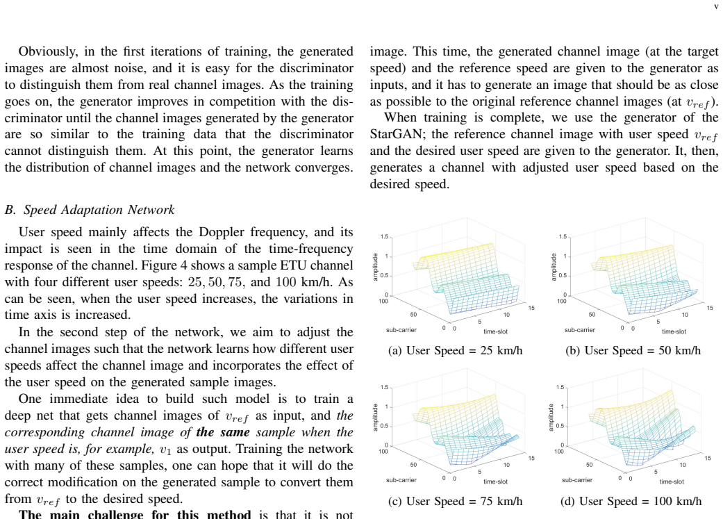
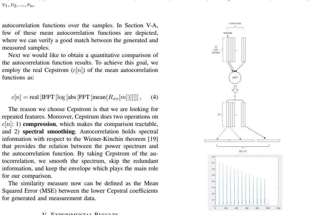
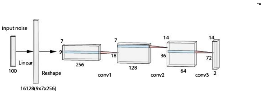
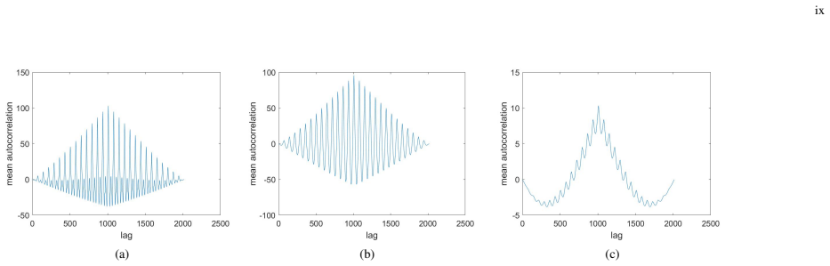
The key objects are (1) the channel image, an m×n×2 array holding real and imaginary parts of the time-frequency response; (2) the channel sample generator, a DCGAN that learns the distribution of these images at a reference speed; (3) the speed adaptation network, a StarGAN that translates images across one-hot speed domains while reconstructing the reference to keep content; and (4) the evaluation metric, which flattens each 2D response into a 1D sequence, averages autocorrelations over samples, takes the real cepstrum of the averaged spectrum, and computes the mean squared error between lower cepstral coefficients.
What would settle it
Compute the same CDM between two independent sets of real measurements of the same channel type and speed; if that within-measurement distance is not substantially smaller than the generated-vs-measured distance, the metric is too lenient to support the similarity claim.
Extended reading notes
Core claim
On its own terms, the paper claims that a two-network generative pipeline — a DCGAN that models the distribution of channel time-frequency images at a reference speed, followed by a StarGAN that adapts the images to other user speeds — yields channel samples statistically equivalent to real measurements. The quantitative evidence is the cepstral distance between the mean autocorrelations of flattened channel grids. In Tables II and III, a generated set is always closest to its own measurement set, typically by an order of magnitude or more, across three simulated channel types and four user speeds.
Load-bearing premise
The cepstral distance between the mean autocorrelations of flattened channel grids is a valid and sufficient measure of statistical similarity for 2D time-frequency responses.
Editorial extensions
If this is right
- A single reference-speed generator plus a StarGAN speed translator can produce channels for multiple speeds without retraining the generative model for each speed.
- The new cepstral-distance metric separates channel types and speeds in a way that LCR and AFD do not, offering a quantitative test for future generative channel models.
- The approach can be applied to both simulated standard channel models (ETU, EVA, PedA) and real Wi-Fi CSI data, suggesting it is not bound to a specific simulation environment.
- Because the pipeline is data-driven, it can in principle model channels whose statistics are hard to express analytically, such as underwater or in-body propagation.
Reading between the lines
- If the CDM is accepted as a similarity measure, the same two-stage pipeline could be applied to other channel parameters such as carrier frequency or bandwidth, or to other propagation media where paired samples are also unavailable.
- The paper's reliance on mean autocorrelation cepstra leaves untested whether the generated images match the full 2D joint distribution; a test using maximum mean discrepancy on the raw images would be a stricter complement.
- The small CDM gap between 75 and 100 km/h suggests the speed translation saturates at high speeds, implying a limit to the speed resolution the network can encode; testing intermediate speeds like 60 or 90 km/h would quantify this.
Signed reviews
Editorial analysis
A structured set of objections, weighed in public.
Referee Report
Summary. The paper proposes a two-stage data-driven model for SISO propagation channels whose time-frequency responses are treated as images. A DCGAN first learns the distribution of channel images at a reference user speed, and a StarGAN then translates these images to other user speeds. The paper introduces a cepstral distance measure (CDM) based on the mean autocorrelation of flattened time-frequency grids, and uses it in Tables II and III to claim that generated channels are statistically similar to the corresponding measurements. Quantitative evaluation is performed on simulated Vienna LTE channels (ETU, EVA, PedA), while a real Wi-Fi CSI experiment is presented only through visual comparison.
Significance. If the statistical-similarity claim were properly supported, the paper would offer a useful and reasonably novel application of GANs to channel modeling: treating the 2D time-frequency response as an image is natural, and using StarGAN for speed adaptation is an elegant way to condition on user speed without paired data. The paper also makes a good-faith attempt to move beyond LCR/AFD by proposing a metric intended to separate channel types and speeds. However, the central claim currently rests on an unvalidated metric and on point estimates without baselines or error bars, and the only quantitative results are for simulated data. Strengths of the paper include its clear problem formulation and the explicit two-stage architecture; the weaknesses are concentrated in the evaluation, which is the load-bearing part of the claim.
major comments (4)
- [§V-A, Tables II and III] The quantitative evidence for the central claim is uncalibrated. The CDM entries are point estimates without error bars, confidence intervals, or a same-type baseline computed from two independent subsets of the measurement data. Consequently, the statement that the diagonal entries are 'an order of magnitude less' than off-diagonal entries is not interpretable, especially because the diagonal entries themselves range from 5.35e-7 to 4.12e-5 in Table II and from 1.43e-5 to 2.98e-5 in Table III. I ask the authors to report bootstrap confidence intervals, to add a measurement-vs-measurement baseline for each channel type and speed, and to state how many measurement and generated realizations are used for each entry.
- [§IV-C, Eq. (4)] The CDM is defined on the cepstrum of the mean autocorrelation of a flattened 1-D concatenation of the 2-D time-frequency grid, but Eq. (4) does not specify how many lower cepstral coefficients are retained, and the text never states the lag range used in Eq. (3). The flattening operation can introduce artificial discontinuities between adjacent rows, and averaging over the flattened sequence may smooth away the joint time-frequency structure that distinguishes channel types or speeds. The authors should validate the CDM on synthetic data with known ground truth, show its sensitivity to the number of cepstral coefficients and to the flattening order, and demonstrate that it captures 2-D joint statistics rather than only per-row or per-column correlations.
- [§V-A, experimental data] The real Wi-Fi CSI experiment is evaluated only visually (Figs. 9(d) and 10(d)); no LCR, AFD, or CDM numbers are reported for it. Since the abstract and Section VI claim statistical similarity to 'measurement data,' the real-data experiment needs quantitative evaluation before the central claim can be accepted. At minimum, report CDM values with baselines for the Wi-Fi data, or clearly restrict the quantitative claim to the simulated Vienna LTE channels.
- [§V-A, Figs. 11 and 12] The LCR/AFD evaluation is incomplete as presented: the text acknowledges that the PedA LCR amplitudes do not match well and that AFD cannot discriminate ETU from EVA even for the actual samples, yet these discrepancies are not quantified. Since LCR/AFD are the only commonly used metrics reported, the authors should include numerical values or a quantitative discrepancy measure, and explain why the observed mismatches do not undermine the claimed statistical similarity.
minor comments (6)
- [§V-A1] In the network-structure paragraph, 'bach size' should be 'batch size'.
- [§IV-C, Eq. (4)] The text uses 'Cepstrom' where 'cepstrum' is intended, and 'Wiener-Kinchin' should be 'Wiener-Khinchin'.
- [§V-B, Fig. 17] The caption and text refer to '50 km/s' in one place; this should be '50 km/h'.
- [§IV-C] The definition of the mean autocorrelation should specify whether the average in Eq. (3) is over samples, over lags, or over both, and should state the maximum lag used in the cepstral computation.
- [Tables II and III] The tables should state the exact number of cepstral coefficients retained and the number of generated/measurement samples used, otherwise the reported numerical values cannot be reproduced or compared across papers.
- [§IV-A] The statement that 'the designed CGAN did not converge properly' is not supported by any training curves or quantitative comparison; a brief description of the attempted CGAN architecture and its failure mode would improve reproducibility.
Circularity Check
No circularity found: the generative model and its CDM evaluation are not equivalent by construction.
full rationale
The paper's derivation chain is self-contained. The channel images are generated by a DCGAN trained with the standard adversarial loss (Eq. 2), and the speed adaptation is performed by StarGAN trained on unpaired real channel images at target speeds; neither training objective uses the evaluation metric as a loss term. The CDM introduced in Section IV-C is an independent post-hoc statistic comparing the cepstra of mean autocorrelations of generated and measured sets. Although the metric is introduced in the same paper and would benefit from calibration and error bars, that is a validation concern, not circularity: the diagonal/off-diagonal comparisons in Tables II and III are not forced by construction, since the generator was not optimized to minimize CDM and the off-diagonal entries use measurements of different channel types or speeds as controls. No self-citations are load-bearing; all external components (StarGAN [17], Vienna simulator [20], Wi-Fi CSI collection [21]) are cited from outside the author team. Hence no step reduces to its own input by definition.
Assumptions & free parameters
free parameters (3)
- number of lower cepstral coefficients used in CDM
- STFT window length and hop size
- reference user speed (v_ref) =
50 km/h for ETU
assumptions (5)
- domain assumption The m x n x 2 channel image representation preserves the statistical information needed for channel modeling.
- domain assumption Simulated data from the Vienna LTE simulator can stand in for real channel measurements when validating the model.
- domain assumption StarGAN's cycle-consistency can learn a valid translation between unpaired channel datasets at different user speeds.
- domain assumption The mean autocorrelation of the flattened time-frequency sequence captures the distinguishing statistics of each channel type and speed.
- standard math Wiener-Khinchin theorem and cepstral smoothing justify using low-order cepstral coefficients of the autocorrelation as a distance metric.
Cite this review
Pith. "Pith review of Propagation Channel Modeling by Deep learning Techniques." pith.science (2026). https://pith.science/paper/33BF7BXA
@misc{pith2026190806767,
  author       = {Pith},
  title        = {Pith review of: Propagation Channel Modeling by Deep learning Techniques},
  year         = {2026},
  howpublished = {\url{https://pith.science/paper/33BF7BXA}},
  note         = {Machine review of arXiv:1908.06767}
}
read the original abstract
Channel, as the medium for the propagation of electromagnetic waves, is one of the most important parts of a communication system. Being aware of how the channel affects the propagation waves is essential for designing, optimization and performance analysis of a communication system. For this purpose, a proper channel model is needed. This paper presents a novel propagation channel model which considers the time-frequency response of the channel as an image. It models the distribution of these channel images using Deep Convolutional Generative Adversarial Networks. Moreover, for the measurements with different user speeds, the user speed is considered as an auxiliary parameter for the model. StarGAN as an image-to-image translation technique is used to change the generated channel images with respect to the desired user speed. The performance of the proposed model is evaluated using existing metrics. Furthermore, to capture 2D similarity in both time and frequency, a new metric is introduced. Using this metric, the generated channels show significant statistical similarity to the measurement data.
Figures


Figures from the paper (13 more)





Forward citations
Cited by 1 Pith paper
-
A Geometry-based Stochastic Wireless Channel Model using Generative Neural Networks
A neural network trained on channel parameters represented as images reproduces the joint statistics of ray-traced wireless channels and beats fully connected baselines on multipath correlation.
Reference graph
Works this paper leans on
-
[1]
A survey of 5g channel measurements and models,
C.-X. Wang, J. Bian, J. Sun, W. Zhang, and M. Zhang, “A survey of 5g channel measurements and models,” IEEE Communications Surveys & Tutorials, vol. 20, no. 4, pp. 3142–3168, 2018
work page 2018
-
[2]
Speed- up techniques for ray tracing field prediction models,
V . Degli-Esposti, F. Fuschini, E. M. Vitucci, and G. Falciasecca, “Speed- up techniques for ray tracing field prediction models,” IEEE Transac- tions on Antennas and Propagation , vol. 57, no. 5, pp. 1469–1480, 2009
work page 2009
-
[3]
Spatial channel model for mimo simulations,
3GPP, “Spatial channel model for mimo simulations,” 2003
work page 2003
-
[4]
An interim channel model for beyond-3g systems: extending the 3gpp spatial channel model (scm),
D. S. Baum, J. Hansen, J. Salo, G. Del Galdo, M. Milojevic, and P. Ky¨osti, “An interim channel model for beyond-3g systems: extending the 3gpp spatial channel model (scm),” in 2005 IEEE 61st V ehicular Technology Conference, vol. 5, pp. 3132–3136, IEEE, 2005
work page 2005
-
[5]
3d extension of the 3gpp/itu channel model,
T. A. Thomas, F. W. V ook, E. Mellios, G. S. Hilton, A. R. Nix, and E. Visotsky, “3d extension of the 3gpp/itu channel model,” in2013 IEEE 77th V ehicular Technology Conference (VTC Spring) , pp. 1–5, IEEE, 2013
work page 2013
-
[6]
Deep learning for massive mimo csi feedback,
C.-K. Wen, W.-T. Shih, and S. Jin, “Deep learning for massive mimo csi feedback,” IEEE Wireless Communications Letters , vol. 7, no. 5, pp. 748–751, 2018
2018
-
[7]
Deep learning for joint source- channel coding of text,
N. Farsad, M. Rao, and A. Goldsmith, “Deep learning for joint source- channel coding of text,” in 2018 IEEE International Conference on Acoustics, Speech and Signal Processing (ICASSP) , pp. 2326–2330, IEEE, 2018
work page 2018
-
[8]
Power of deep learning for channel estimation and signal detection in ofdm systems,
H. Ye, G. Y . Li, and B.-H. Juang, “Power of deep learning for channel estimation and signal detection in ofdm systems,” IEEE Wireless Communications Letters , vol. 7, no. 1, pp. 114–117, 2018
work page 2018
Show all 21 references
-
[9]
Generative adversarial nets,
I. Goodfellow, J. Pouget-Abadie, M. Mirza, B. Xu, D. Warde-Farley, S. Ozair, A. Courville, and Y . Bengio, “Generative adversarial nets,” in Advances in neural information processing systems , pp. 2672–2680, 2014
2014
-
[10]
Unsupervised representation learning with deep convolutional generative adversarial networks,
A. Radford, L. Metz, and S. Chintala, “Unsupervised representation learning with deep convolutional generative adversarial networks,”arXiv preprint arXiv:1511.06434, 2015
2015 arXiv
-
[11]
Conditional generative adversarial nets for convolutional face generation,
J. Gauthier, “Conditional generative adversarial nets for convolutional face generation,” Class Project for Stanford CS231N: Convolutional Neural Networks for Visual Recognition, Winter semester , vol. 2014, no. 5, p. 2, 2014
2014
-
[12]
Began: Boundary equilib- rium generative adversarial networks,
D. Berthelot, T. Schumm, and L. Metz, “Began: Boundary equilib- rium generative adversarial networks,”arXiv preprint arXiv:1703.10717, 2017
2017 arXiv
-
[13]
Improved training of wasserstein gans,
I. Gulrajani, F. Ahmed, M. Arjovsky, V . Dumoulin, and A. C. Courville, “Improved training of wasserstein gans,” in Advances in Neural Infor- mation Processing Systems , pp. 5767–5777, 2017
2017
-
[14]
Image-to-image translation with conditional adversarial networks,
P. Isola, J.-Y . Zhu, T. Zhou, and A. A. Efros, “Image-to-image translation with conditional adversarial networks,” in Proceedings of the IEEE conference on computer vision and pattern recognition , pp. 1125–1134, 2017
2017
-
[15]
Unpaired image-to-image translation using cycle-consistent adversarial networks,
J.-Y . Zhu, T. Park, P. Isola, and A. A. Efros, “Unpaired image-to-image translation using cycle-consistent adversarial networks,” in Proceedings of the IEEE international conference on computer vision , pp. 2223– 2232, 2017
2017
-
[16]
Dual generator genera- tive adversarial networks for multi-domain image-to-image translation,
H. Tang, D. Xu, W. Wang, Y . Yan, and N. Sebe, “Dual generator genera- tive adversarial networks for multi-domain image-to-image translation,” arXiv preprint arXiv:1901.04604 , 2019
1901 arXiv
-
[17]
Stargan: Unified generative adversarial networks for multi-domain image-to- image translation,
Y . Choi, M. Choi, M. Kim, J.-W. Ha, S. Kim, and J. Choo, “Stargan: Unified generative adversarial networks for multi-domain image-to- image translation,” in Proceedings of the IEEE Conference on Computer Vision and Pattern Recognition , pp. 8789–8797, 2018
2018
-
[18]
Deep learning-based channel estimation for beamspace mmwave massive mimo systems,
H. He, C.-K. Wen, S. Jin, and G. Y . Li, “Deep learning-based channel estimation for beamspace mmwave massive mimo systems,” IEEE Wireless Communications Letters , vol. 7, no. 5, pp. 852–855, 2018
2018
-
[19]
R. D. Yates and D. J. Goodman, Probability and stochastic processes: a friendly introduction for electrical and computer engineers . John Wiley & Sons, 2014
2014
-
[20]
M. Rupp, S. Schwarz, and M. Taranetz, The Vienna LTE-advanced simulators. Springer, 2016
2016
-
[21]
Precise power delay profiling with commodity wifi,
Y . Xie, Z. Li, and M. Li, “Precise power delay profiling with commodity wifi,” in Proceedings of the 21st Annual International Conference on Mobile Computing and Networking , MobiCom ’15, (New York, NY , USA), p. 5364, ACM, 2015
2015
Reviewed August 14, 2026 · model on record in the stance chip above.
Discussion (0). Continue with ORCID to comment.