Pith. sign in

REVIEW 3 major objections 3 minor

From Approximation to Emergence: A Theory of Deep Learning

T0 review · 3 major / 3 minor · reviewed 2026-08-02 · deepseek-v4-flash

Pith's one-line read This monograph argues that modern deep learning theory can be organized into a single coherent narrative, from approximation and optimization to the open question of emergence.

desk verdict A clear, honest abstract for a book that promises a useful map of DL theory; the map may be real, but an abstract alone is not enough to referee. read the letter →

arxiv 2607.01311 v2 pith:36L3KIOK submitted 2026-07-01 cs.LG stat.ML

classification cs.LGstat.ML MSC 68T07
keywords deeplearningtheoryapproximationoptimizationgeneralizationtransformersin-contextemergenceresearchnarrative
verification ladder T0 review T1 audit T2 compute T3 formal

The pith

A machine-rendered reading of the paper's core claim, the machinery that carries it, and where it could break.

The reading

The book's central claim is that deep learning theory is not a disconnected set of results but a unified research story that can be traced from classical approximation, optimization, and generalization to contemporary topics like transformers, in-context learning, scaling laws, and emergence. It proposes a recurring three-question frame for understanding any theoretical result: what object the theory controls, what assumptions make it valid, and what phenomena it leaves unexplained. If this framing holds, researchers and students gain a structured map of the field, with gaps and open problems appearing in systematic places. The author positions emergence as the culminating open question: how learned mechanisms arise from scale, data, architecture, and training.

What carries the argument

The organizing device is the three-question frame: for any theory, identify the object it controls, the assumptions under which it is valid, and the unexplained phenomena it leaves behind. This frame is meant to turn a fragmented literature into a coherent narrative and to locate emergence as the central open problem.

What would settle it

Pick any chapter and check whether it actually presents each theory in the claimed three-part form; if a major subfield is covered as isolated theorems without identifying the object controlled, the assumptions, and the left-out phenomena, the book's unifying claim fails for that part of the literature.

Watch

Extended reading notes

Core claim

The paper's central claim is that a proof-oriented, unified account of deep learning theory is possible, and that the book delivers it by organizing the literature into a coherent narrative. Each theory is examined through three questions: the object it controls, the assumptions that make it valid, and the phenomena it leaves unexplained. This three-question frame is applied across a path that starts with approximation, optimization, and generalization, then moves through overparameterization, robustness, generative modeling, transformers, in-context learning, scaling laws, interpretability, alignment, and emergence.

Load-bearing premise

The book's unity claim depends on the assumption that a single narrative can genuinely connect all the listed subfields, each with proof-oriented theories, even though emergence is itself an unresolved open question.

Editorial extensions

If this is right

  • If the frame works, every deep learning theory can be described in comparable terms, exposing shared structure and hidden gaps across subfields.
  • Unexplained phenomena become an explicit part of each theory's description, making open problems a systematic output of the narrative rather than an afterthought.
  • The book gives graduate students and researchers a single map of the field, from classical foundations to frontier topics.
  • Emergence is cast as the unresolved question that ties together scale, data, architecture, and training, pointing future work toward explaining how learned mechanisms arise.

Reading between the lines

Editorial extensions of the paper, not claims the author makes directly.

  • One could test the frame's usefulness by taking recent papers outside the book's list, such as mechanistic interpretability or safety research, and seeing whether they naturally fit the object/assumptions/unexplained-phenomena trichotomy.
  • The narrative implies that scaling laws and in-context learning are partial milestones toward explaining emergence, but the author leaves it open whether these are genuinely explanatory or just phenomenological descriptions.
  • If the frame is accepted, a natural next step is to build a taxonomy of unexplained phenomena across subfields, which could guide new theoretical work toward the open question of emergence.
Share X Bluesky LinkedIn Reddit HN

Signed reviews

No signed human review yet.

Editorial analysis

A structured set of objections, weighed in public.

Desk editor's note, referee report, and a circularity audit.

Referee Report

3 major / 3 minor

Summary. The manuscript under review is a book abstract for 'From Approximation to Emergence: A Theory of Deep Learning.' It promises a unified, proof-oriented survey of deep learning theory, organized through a three-question frame (the object each theory controls, the assumptions that make it valid, and the phenomena it leaves unexplained). The abstract lists coverage from classical approximation, optimization, and generalization to contemporary topics including overparameterization, robustness, generative modeling, transformers, in-context learning, scaling laws, interpretability, alignment, and emergence. Only the abstract is available for review; no chapters, equations, references, or proof sketches are provided.

Significance. If the book delivers on its promise, it would be a valuable synthesis: a single map of deep learning theory with a consistent analytical lens could help researchers and students navigate a fragmented literature. The abstract is candid that the field is 'incomplete' and that emergence is an open question, which is a sign of balance. However, the abstract alone cannot establish the claimed proof-oriented character or the coherence of the narrative. No machine-checked proofs, reproducible code, or parameter-free derivations are present in the reviewable material; 'proof-oriented' is a promise, not a demonstrated property. The significance therefore depends entirely on execution that is not currently verifiable.

major comments (3)
  1. [Abstract (central claim)] The manuscript's central assertion—a 'unified, proof-oriented account'—is not checkable from the abstract. The abstract lists topics and states an organizing frame, but it does not differentiate theorem-backed results from conceptual surveys. If the book's chapters contain formal results for all listed areas, the claim may hold; if some chapters are literature reviews or open-problem statements, the 'proof-oriented' label overstates the content. This is load-bearing because the title and framing rest on it. As provided, the claim can be neither confirmed nor refuted.
  2. [Abstract (emergence)] The abstract itself characterizes emergence as an open question 'increasingly centered on the question of how learned mechanisms arise.' That phrasing suggests the emergence chapter may primarily organize open problems rather than present theorems. If so, the unified 'proof-oriented account' is uneven: classical areas may have rigorous theories while emergence, interpretability, and alignment may not. The abstract should either explicitly qualify the proof-oriented claim (e.g., 'proof-oriented where results exist') or indicate the formal status of these chapters. The title's path 'to emergence' makes this point central rather than peripheral.
  3. [Abstract (coherence frame)] The three-question frame—object controlled, assumptions made, phenomena left unexplained—is a reasonable expository device, but it does not by itself establish a 'coherent research narrative' or a unified theory. Different subfields may have different mathematical objects and assumptions, and the abstract does not say what ties them together beyond the shared frame. If the book is a sequence of separate surveys, the claimed unification is largely rhetorical. A sentence specifying the overarching connection (e.g., a common mathematical formalism, a shared notion of learned mechanisms, or a developmental narrative) would help assess the claim.
minor comments (3)
  1. [Abstract (terminology)] The term 'proof-oriented' should be defined. Does it mean 'contains proofs,' 'organized around theorems,' or 'theories that have been proven in simplified settings'? Without a definition, readers cannot evaluate the scope.
  2. [Abstract (scope clarity)] The abstract would benefit from a chapter list or a table of contents, even a condensed one, so that the claimed path from approximation to emergence is visible. This would also make the reviewable artifact more informative.
  3. [Abstract (interpretability and alignment)] The abstract groups interpretability and alignment with areas that have developed formal theories. It would clarify the book's contribution to state whether these chapters present formal guarantees, empirical observations, or a combination.

Circularity Check

0 steps flagged · score 0.0 of 10

No circularity found in abstract; no derivation chain to reduce.

full rationale

This is an abstract-only review, and the abstract contains no derivation chain, no equations, no fitted parameters, no self-citations, and no empirical predictions that could be circular. Its organizing claim—that each theory is examined through the object it controls, the assumptions that make it valid, and the phenomena it leaves unexplained—is an expository framing device, not a derivation that reduces to its own inputs. The abstract explicitly characterizes emergence as an open question 'increasingly centered on the question of how learned mechanisms arise,' which is honest about the limits of the surveyed field rather than presenting a conclusion as forced. Any concern about whether the book actually delivers proof-oriented coverage of every listed subfield is a question of scope or correctness, not circularity under the defined patterns. No specific circular step can be quoted because none exists in the available text.

Assumptions & free parameters 0 free parameters · 3 assumptions · 0 invented entities

No numerical free parameters exist in an abstract-only review; the book's contribution is organizational, not derivational. The load-bearing assumptions are about the accuracy and the unity of the proposed narrative. The 'object it controls / assumptions / unexplained phenomena' structure is an editorial lens, not a fitted parameter or invented entity.

assumptions (3)
  • domain assumption The cited results in approximation, optimization, generalization, and the modern subfields are correctly characterized in the monograph.
    The abstract promises a 'proof-oriented account' of a broad literature; accuracy of these characterizations is the core of the book's value and is unverifiable from the abstract alone.
  • ad hoc to paper A single narrative can coherently organize the listed subfields into one path.
    The abstract's central organizing claim is that the field can be traced as one coherent story; this unity is a thematic premise of the book, not a fact established by the abstract.
  • domain assumption Phenomena labeled 'emergence' are amenable to mathematical 'theory' at all.
    The abstract itself concedes the field is 'incomplete' and centered on the open question of how mechanisms arise; treating emergence as the narrative's endpoint assumes there is theory worth mapping there.

how reviews work

0 comments
Cite this review

Pith. "Pith review of From Approximation to Emergence: A Theory of Deep Learning." pith.science (2026). https://pith.science/paper/36L3KIOK

@misc{pith2026260701311,
  author       = {Pith},
  title        = {Pith review of: From Approximation to Emergence: A Theory of Deep Learning},
  year         = {2026},
  howpublished = {\url{https://pith.science/paper/36L3KIOK}},
  note         = {Machine review of arXiv:2607.01311}
}
read the original abstract

Deep learning has outgrown any single mathematical explanation. From Approximation to Emergence develops a unified, proof-oriented account of modern deep learning theory, tracing a path from the classical foundations of approximation, optimization, and generalization to the contemporary mechanisms of overparameterization, robustness, generative modeling, transformers, in-context learning, scaling laws, interpretability, alignment, and emergence. Rather than presenting isolated results, the book organizes a broad literature into a coherent research narrative: each theory is examined through the object it controls, the assumptions that make it valid, and the phenomena it leaves unexplained. Written for researchers, graduate students, and mathematically trained practitioners, this monograph offers a rigorous map of deep learning theory as it stands today: powerful, incomplete, and increasingly centered on the question of how learned mechanisms arise from scale, data, architecture, and training.

Figures
Figures reproduced from arXiv: 2607.01311 by the authors.

Figure 2.1
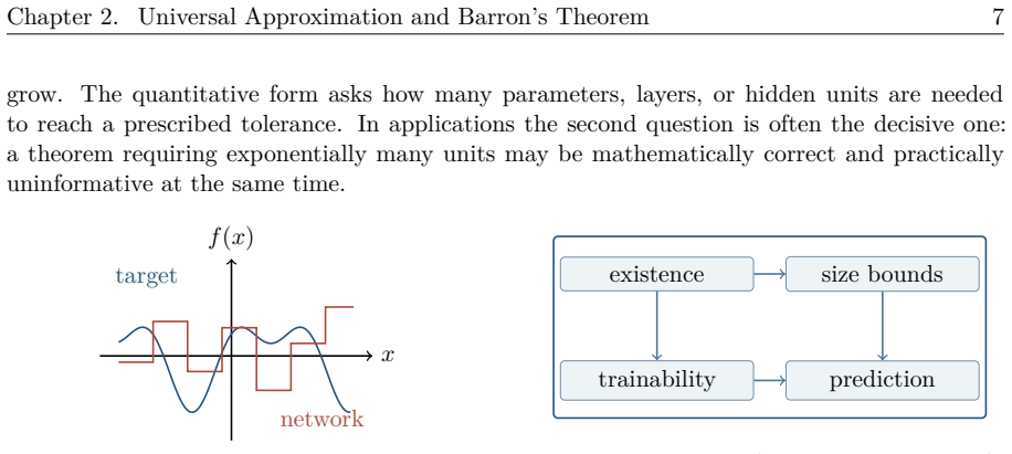
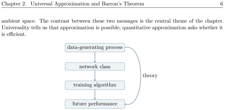
Figure 2.1. A useful theory must connect the data-generating process, the model class, the training algorithm, and performance on future data. The monograph will repeatedly return to four lenses: approximation, optimization, gener￾alization, and representation. Approximation asks which functions can be represented, and at what size. Optimization asks whether an algorithm can locate a good representative of the class. Generaliza… view at source ↗
Figure 2.2
Figure 2.2. Mathematical theory tries to move from fitting labels to predictions with explicit guarantees. Approximation Which functions can networks represent? Optimization Can algorithms find them? Generalization Why predict on new data? Representation What structure is learnable? deep learning theory [PITH_FULL_IMAGE:figures/full_fig_p015_2_2.png] view at source ↗
Figure 2.5
Figure 2.5. Universal approximation is only a starting point. It does not by itself give size, optimization, or prediction guarantees. 2.2 The Learning Setup We now introduce the statistical notation used throughout the chapter. Let µ be an unknown distribution on R d × Y. A training sample is S = {(xi , yi)} n i=1, (xi , yi) ∼ µ, typically assumed independent and identically distributed. The vector xi ∈ R d contains the observ… view at source ↗
Figures from the paper (354 more)
Figure 2.6
Figure 2.6. Figure 2.6: The training data are samples from an unknown distribution. Definition 2.1 (Population and Empirical Risk). Given a loss ℓ(y, y b ), the population risk and empirical risk are R(f) = E(x,y)∼µ [PITH_FULL_IMAGE:figures/full_fig_p016_2_6.png]
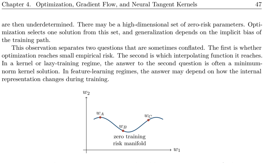
Figure 2.8
Figure 2.8. Figure 2.8: A nonlinear rule in the original coor￾dinates can become a linear rule after a feature map, for example ϕ(x) = (x1, x2, x2 1 , x2 2 , x1x2) >. The approximation problem may now be stated abstractly. Given a target function g and a network class FL,m of depth L and wi…
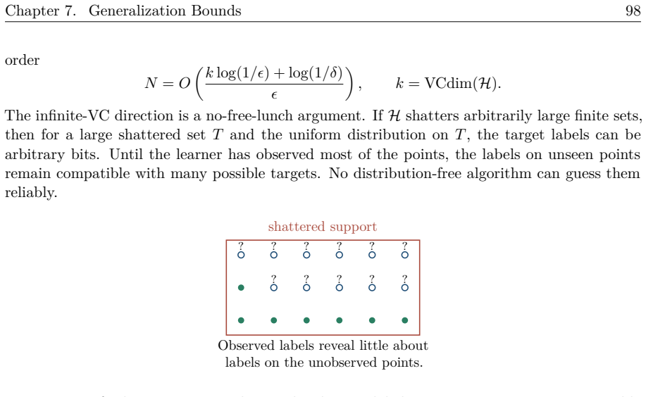
Figure 2.9
Figure 2.9. Figure 2.9: A feedforward network composes layers of affine maps and coordinatewise nonlin￾earities. The choice of activation matters. Standard examples include ReLU(t) = max{t, 0}, s(t) = 1 1 + e−t , H(t) = 1{t≥0} , c(t) = cos(t). ReLU activations give continuous piecewise-line…
Figure 2.10
Figure 2.10. Figure 2.10: Three basic activations: ReLU, sigmoid, and threshold. these partitions. This remark is often the most useful way to remember ReLU expressivity. A single ReLU unit ReLU(hw, xi + b) is affine on each side of the hyperplane hw, xi + b = 0. A sum of such units creates …
Figure 2.11
Figure 2.11. Figure 2.11: A one-dimensional ReLU network is piecewise linear; the dashed lines mark hinge locations. expressivity control structured classes uncontrolled fitting [PITH_FULL_IMAGE:figures/full_fig_p020_2_11.png]
Figure 2.12
Figure 2.12. Figure 2.12: More expressivity is valuable only when accompanied by mathematical control. 2.4 Universal Approximation Definition 2.4 (Universal Approximator). Let K ⊂ R d be compact. A function class F ⊂ C(K) is a universal approximator if, for every g ∈ C(K) and every ε > 0, th…
Figure 2.13
Figure 2.13. Figure 2.13: A continuous target can first be approximated by simple local pieces. Proposition 2.7 (Lipschitz Step Approximation). Let g : [0, 1] → R be ρ-Lipschitz and let H(t) = 1{t≥0} . For every ε > 0, there is a depth-two threshold network gb(x) = g(0) + mX−1 i=1 [PITH_FUL…
Figure 2.14
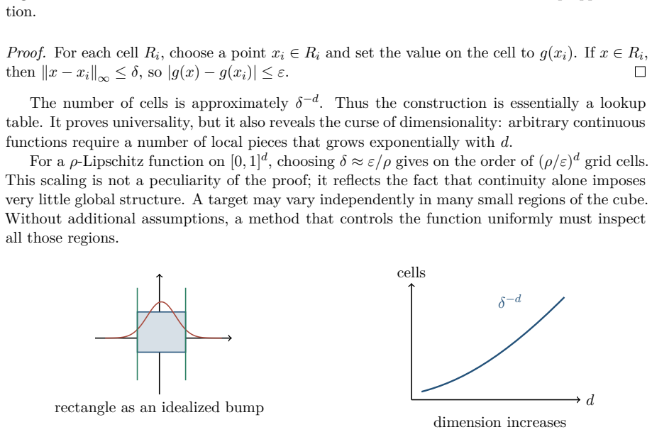
Figure 2.14. Figure 2.14: The one-dimensional construction uses threshold units to build a step approxima￾tion. Proof. For each cell Ri , choose a point xi ∈ Ri and set the value on the cell to g(xi). If x ∈ Ri , then kx − xik∞ ≤ δ, so |g(x) − g(xi)| ≤ ε. The number of cells is approximately…
Figure 2.15
Figure 2.15. Figure 2.15: In several dimensions, local pieces are rectangle-like bumps. d cells δ −d dimension increases [PITH_FULL_IMAGE:figures/full_fig_p023_2_15.png]
Figure 2.17
Figure 2.17. Figure 2.17: The Barron seminorm penalizes Fourier mass far from the origin. measure on K. If B(f) < ∞, then for every k ≥ 1 there exists a depth-two network fk(x) = X k j=1 aj σ(hwj , xi + bj ) such that Z K |f(x) − fk(x)| 2 dµ(x) ≤ C B(f) 2 k , where C depends on normalization…
Figure 2.18
Figure 2.18. Figure 2.18: An infinite-width representation averages ridge features over a distribution. integral rep￾resentation sample k units finite O network (k −1/2) [PITH_FULL_IMAGE:figures/full_fig_p026_2_18.png]
Figure 2.20
Figure 2.20. Figure 2.20: Barron’s proof rewrites the target as an infinite-width network and sparsifies the integral. Example 2.13 (Low and High Frequencies). For a unit direction u, f(x) = cos(2π u>x) has Fourier mass concentrated at ±u, so its Barron quantity scales with kuk. By contrast,…
Figure 2.21
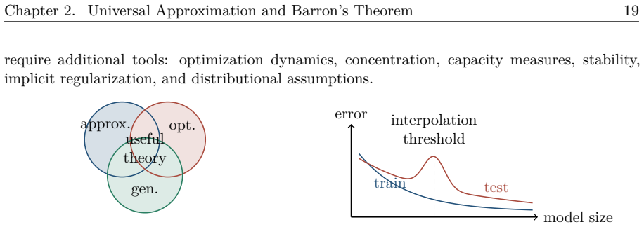
Figure 2.21. Figure 2.21: Fourier spikes farther from the origin increase the Barron quantity. 2.6 Connections and Limits Approximation theorems are necessary but not sufficient explanations of deep learning. They tell us that a good network exists; optimization asks whether training finds o…
Figure 2.22
Figure 2.22. Figure 2.22: Useful theory connects ap￾proximation, optimization, and general￾ization. model size error train test interpolation threshold [PITH_FULL_IMAGE:figures/full_fig_p028_2_22.png]
Figure 2.24
Figure 2.24. Figure 2.24: Depth can encode hierarchical or compositional structure succinctly. There is also a complementary width-versus-depth result. For ReLU networks with un￾bounded depth, narrow architectures can still be universal in L p senses. A representative [PITH_FULL_IMAGE:figur…
Figure 3.1
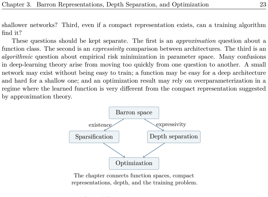
Figure 3.1. Figure 3.1: The conceptual flow of Chapter 2. Barron theory gives a representation and a finite-width approximation mechanism. Depth separation gives a different kind of expressivity result. Optimization asks whether the useful representation can be found from data. A useful men…
Figure 3.2
Figure 3.2. Figure 3.2: The shallow-network mental model. Each hidden unit is a ridge feature, and the theorem explains when a finite number of such features is enough. How to Read This Chapter The first two sections study shallow approximation: an analytic condition on f gives an infinite …
Figure 3.3
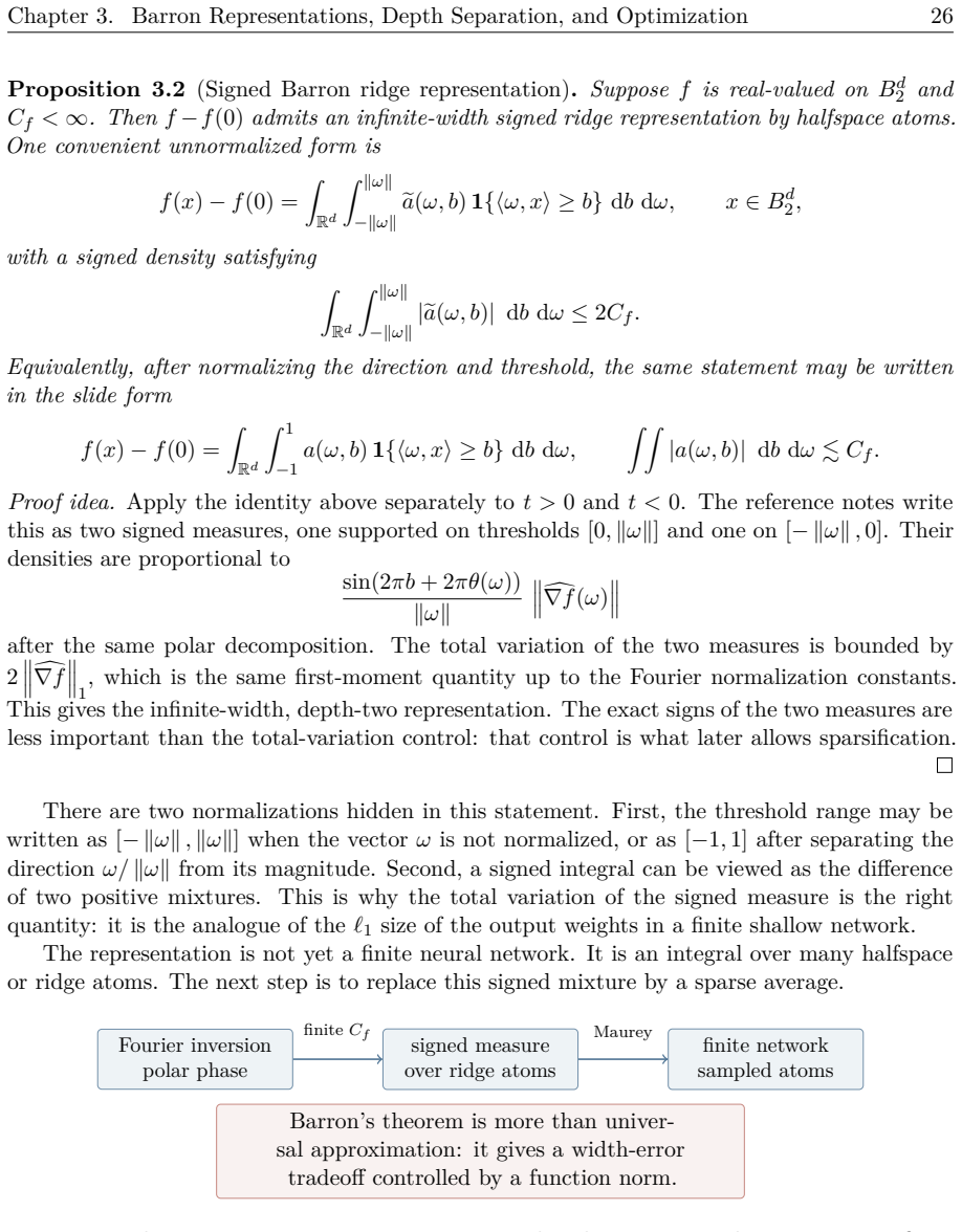
Figure 3.3. Figure 3.3: A Fourier mode is a sinusoid along the direction ω. By subtracting f(0) and integrating along the scalar variable hω, xi, one obtains ridge-type threshold atoms. 3.2.1 From Fourier Phase to Halfspace Atoms The starting point is to subtract the constant value f(0). Fr…
Figure 3.4
Figure 3.4. Figure 3.4: The representation-to-approximation path. The Fourier condition gives an infinite signed mixture, and sparsification converts that mixture into a finite shallow network. The passage from indicator atoms to ReLU atoms is conceptually simple. In one dimension, (t)+ = Z…
Figure 3.5
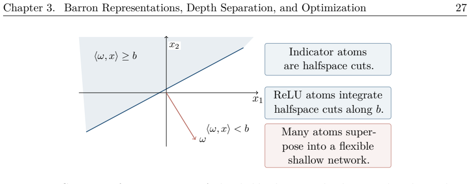
Figure 3.5. Figure 3.5: Geometry of a Barron atom. A threshold ridge atom divides space by a hyperplane; ReLU ridge functions can be viewed as integrated threshold atoms. Representation Versus Approximation The signed integral is an exact infinite-width representation. The finite network ob…
Figure 3.6
Figure 3.6. Figure 3.6: Gaussian spectrum intuition. Most mass remains near the origin, and the first spectral moment grows like the typical radius of a Gaussian vector. Rates for nonparametric estimation often degrade with dimension through volume effects. Bar￾ron approximation is a differ…
Figure 3.7
Figure 3.7. Figure 3.7: Frank-Wolfe sparsification. The target X lies in the convex hull of atoms; each greedy step adds one atom while staying inside the hull. Proof. As in Maurey’s lemma, write X = E[V ] for a random atom V ∈ S. Because the greedy step is at least as good as choosing a ra…
Figure 3.8
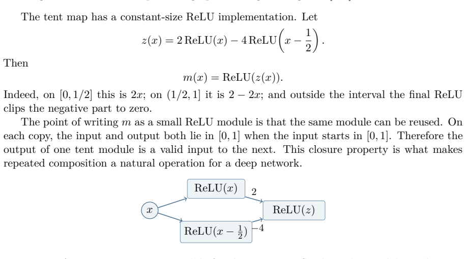
Figure 3.8. Figure 3.8: The tent map m. Its graph is a single triangle on [0, 1] and zero outside. The tent map has a constant-size ReLU implementation. Let z(x) = 2 ReLU(x) − 4 ReLU x − 1 2  . Then m(x) = ReLU(z(x)). Indeed, on [0, 1/2] this is 2x; on (1/2, 1] it is 2 − 2x; and outside t…
Figure 3.9
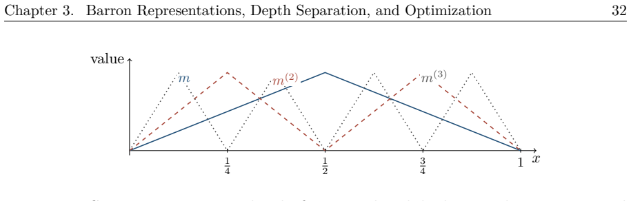
Figure 3.9. Figure 3.9: A constant-size ReLU module for the tent map. Stacking this module implements iterates of m. The key phenomenon appears when we compose m with itself. Write m(k) = m| ◦ m {z ◦ · · · ◦ m} k times . Each iteration doubles the number of teeth on [0, 1]. Thus m(k) has 2 …
Figure 3.10
Figure 3.10. Figure 3.10: Composition creates teeth. The first, second, and third iterates have one, two, and four teeth on [0, 1]. 3.4.2 Sawtooth Complexity Definition 3.6 (t-sawtooth function). A univariate function f : R → R is t-sawtooth if its domain can be partitioned into at most t in…
Figure 3.11
Figure 3.11. Figure 3.11: A schematic for the sawtooth counting bound. ReLU units create piecewise-affine maps; depth composes these maps. 3.4.3 Telgarsky’s Separation Theorem 3.9 (Telgarsky depth separation). For every sufficiently large L, there exists a function f : [0, 1] → [0, 1] comput…
Figure 3.12
Figure 3.12. Figure 3.12: Deep implementation by module reuse. The tent-map module is small; iterating it produces an exponentially oscillatory function. The proof picture is the following. The target f = m(L2+2) has roughly 2 L2+2 small triangles. A shallow network g, because it has only li…
Figure 3.13
Figure 3.13. Figure 3.13: Missing triangles. A shallow piecewise-affine approximator cannot track every oscillation of an iterated tent map. triangles are missed. This gives Z 1 0 |f(x) − g(x)| dx ≥ 1 2 [PITH_FULL_IMAGE:figures/full_fig_p043_3_13.png]
Figure 3.14
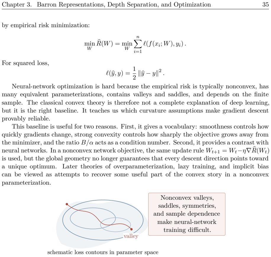
Figure 3.14. Figure 3.14: A schematic nonconvex loss landscape. The slide used a surface plot; the essential point is the same: neural-network objectives are not simple convex bowls. 3.5.1 Convex Functions and Gradient Descent Definition 3.11 (Convex function). A differentiable function F : …
Figure 3.15
Figure 3.15. Figure 3.15: Gradient descent geometry in the convex baseline theory. The iterates move through nested sublevel sets toward the minimizer. Definition 3.12 (B-smoothness). A differentiable function F is B-smooth if k∇F(x) − ∇F(y)k ≤ B kx − yk for all x, y. If F is twice different…
Figure 3.16
Figure 3.16. Figure 3.16: A concept map for later chapters. Approximation, generalization, and optimization will remain separate but interacting themes. Remark 3.15 (Limitations and open directions). Barron bounds are strongest for functions with small spectral first moment. Telgarsky’s cons…
Figure 4.1
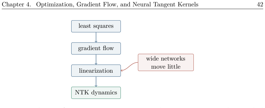
Figure 4.1. Figure 4.1: The route from convex optimization to NTK theory. Least squares explains residual flow with a fixed feature matrix; NTK analysis repeats the same algebra with the neural-network Jacobian. the parameters move only a little, so the network remains close to its tangent …
Figure 4.2
Figure 4.2. Figure 4.2: The smallest positive eigenvalue of the relevant kernel controls the slowest residual direction. A larger spectral gap gives faster decay. 4.1.1 Finite-Sample Setup Fix a training set {(xi , yi)} N i=1 and parameters w ∈ R p . It is convenient to suppress the input p…
Figure 4.3
Figure 4.3. Figure 4.3: Parameter space and prediction space. NTK analysis studies a nonconvex parameter trajectory through the induced ODE on the finite vector of training predictions. 4.2 Least Squares and Gradient Flow Before neural networks, we analyze the model problem min x F(x) = 1 2…
Figure 4.4
Figure 4.4. Figure 4.4: Least-squares geometry. Under strong convexity the contours are elliptic bowls, and gradient descent moves toward the unique minimizer. 4.2.1 Residual Dynamics Let rt = Axt − b. Gradient descent with stepsize η gives xt+1 = xt − ηA>rt . Multiplying by A converts the …
Figure 4.5
Figure 4.5. Figure 4.5: The least-squares Gram matrix. The smallest eigenvalue determines the slowest residual direction. This warm-up matters because the same algebra reappears with A ←→ J(w(0)). The linearized neural network is a least-squares problem whose feature matrix is the Jacobian …
Figure 4.6
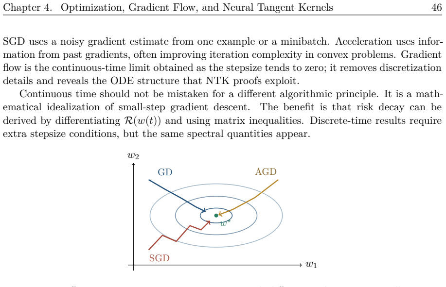
Figure 4.6. Figure 4.6: Different optimization trajectories can reach different endpoints, especially in non￾convex overparameterized models. 4.3 Nonconvexity and Overparameterization Beyond convexity, several reassuring implications break. Global minimization is computation￾ally hard in ge…
Figure 4.7
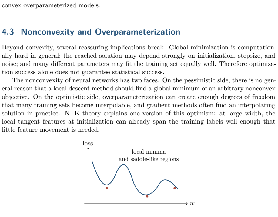
Figure 4.7. Figure 4.7: A schematic nonconvex objective. Gradient methods may be easy to run but hard to analyze globally. In overparameterized neural networks, p N is common. The interpolation equations f(xi ; w) = yi , i = 1, . . . , N, [PITH_FULL_IMAGE:figures/full_fig_p055_4_7.png]
Figure 4.8
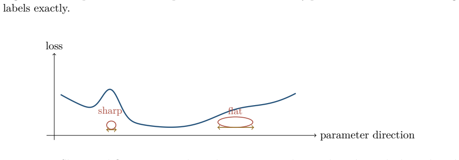
Figure 4.8. Figure 4.8: Interpolation in an overparameterized model. Many parameters can fit the training labels exactly. parameter direction loss sharp flat [PITH_FULL_IMAGE:figures/full_fig_p056_4_8.png]
Figure 4.9
Figure 4.9. Figure 4.9: Sharp and flat minima. The endpoint matters, but so does the path that selected it. This is the setting in which one would like a theorem of the following form: for a fixed training set of size N, a sufficiently wide randomly initialized network reaches zero training…
Figure 4.10
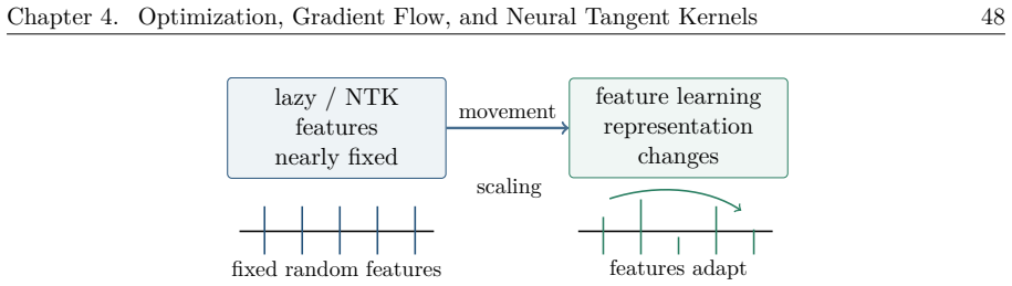
Figure 4.10. Figure 4.10: The tension between kernel learning and feature learning. NTK theory analyzes a regime where tangent features remain nearly fixed. fine Jt =    ∇wf(x1; w(t))> . . . ∇wf(xN ; w(t))>    ∈ R N×p . The empirical neural tangent kernel is Kt = JtJ > t , Kt(i, j) = h…
Figure 4.11
Figure 4.11. Figure 4.11: Linearization at initialization. Lazy training analyzes the network near w0, replac￾ing it by its tangent model. 4.4.2 Linearization at Initialization Near w0 = w(0), define the affine approximation f0(u) = f(w0) + J0(u − w0), J0 = J(w0). The corresponding linearize…
Figure 4.12
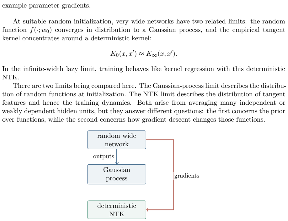
Figure 4.12. Figure 4.12: The empirical NTK as a Gram matrix. Its entries are inner products of training￾example parameter gradients. At suitable random initialization, very wide networks have two related limits: the random function f(·; w0) converges in distribution to a Gaussian process, a…
Figure 4.13
Figure 4.13. Figure 4.13: Random networks give both Gaussian-process output limits and deterministic tangent-kernel limits under appropriate width and scaling. 4.5 Convergence Mechanisms 4.5.1 Fixed-Kernel Decay For the linearized flow, the kernel K0 is constant: r˙(t) = −α 2K0r(t), r(t) = e…
Figure 4.14
Figure 4.14. Figure 4.14: The bootstrap structure of lazy-training proofs. Assume kernel stability, prove small movement, then use small movement and width to justify kernel stability. 4.6 Random Features, Adaptive Features, and Width The simplest model behind the NTK proof is a random-featu…
Figure 4.15
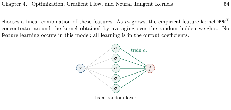
Figure 4.15. Figure 4.15: Random features. The hidden features are sampled once and held fixed, so the optimization problem is linear in the output weights. For a two-layer neural network with trainable hidden features, f(x; w) = 1 √ m Xm r=1 arσ(b > r x), the tangent kernel has two types of…
Figure 4.16
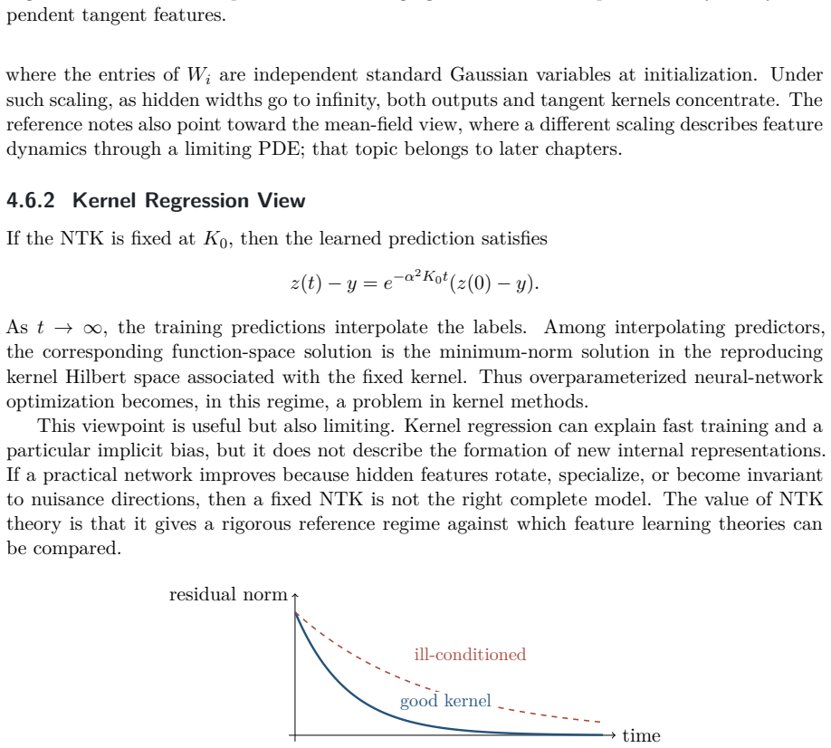
Figure 4.16. Figure 4.16: Width as duplication and averaging. Wider networks provide many nearly inde￾pendent tangent features. where the entries of Wi are independent standard Gaussian variables at initialization. Under such scaling, as hidden widths go to infinity, both outputs and tangent…
Figure 4.17
Figure 4.17. Figure 4.17: Kernel-flow residual decay. A well-conditioned kernel removes residual components quickly; an ill-conditioned kernel has slow directions. 4.7 What NTK Theory Explains NTK theory explains why sufficiently wide random networks can fit finite training sets, why least-s…
Figure 5.1
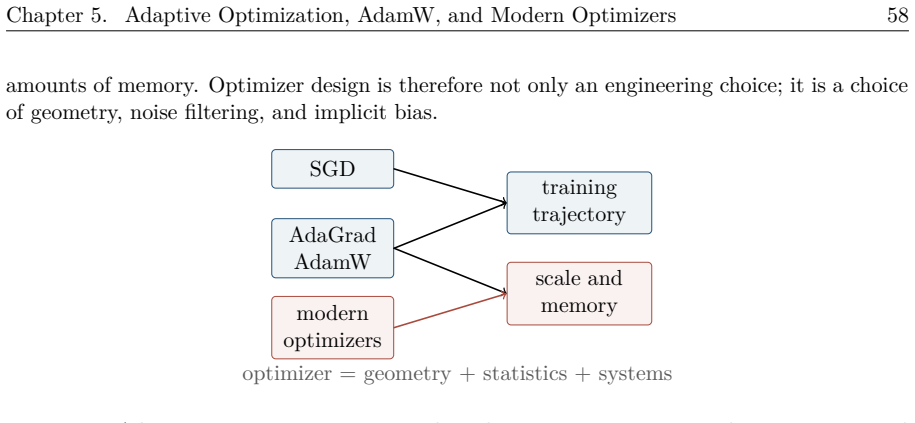
Figure 5.1. Figure 5.1: Adaptive optimization connects algorithmic geometry, noisy gradient statistics, and the practical cost of training foundation models. The guiding question is: How do adaptive optimizers change geometry, implicit bias, and the cost of training foundation models? The a…
Figure 5.2
Figure 5.2. Figure 5.2: The inserted chapter bridges optimization dynamics and implicit regularization by asking how the optimizer changes the path to interpolation. Definition 5.1 (Preconditioned stochastic descent). Let f(θ) = Eξ∼Dℓ(θ; ξ), gt ≈ ∇f(θt) be a stochastic gradient. A precondit…
Figure 5.3
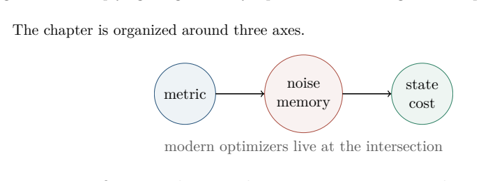
Figure 5.3. Figure 5.3: Multiplying the gradient by a preconditioner changes the steepest descent direction. The chapter is organized around three axes. metric noise memory state cost modern optimizers live at the intersection [PITH_FULL_IMAGE:figures/full_fig_p068_5_3.png]
Figure 5.4
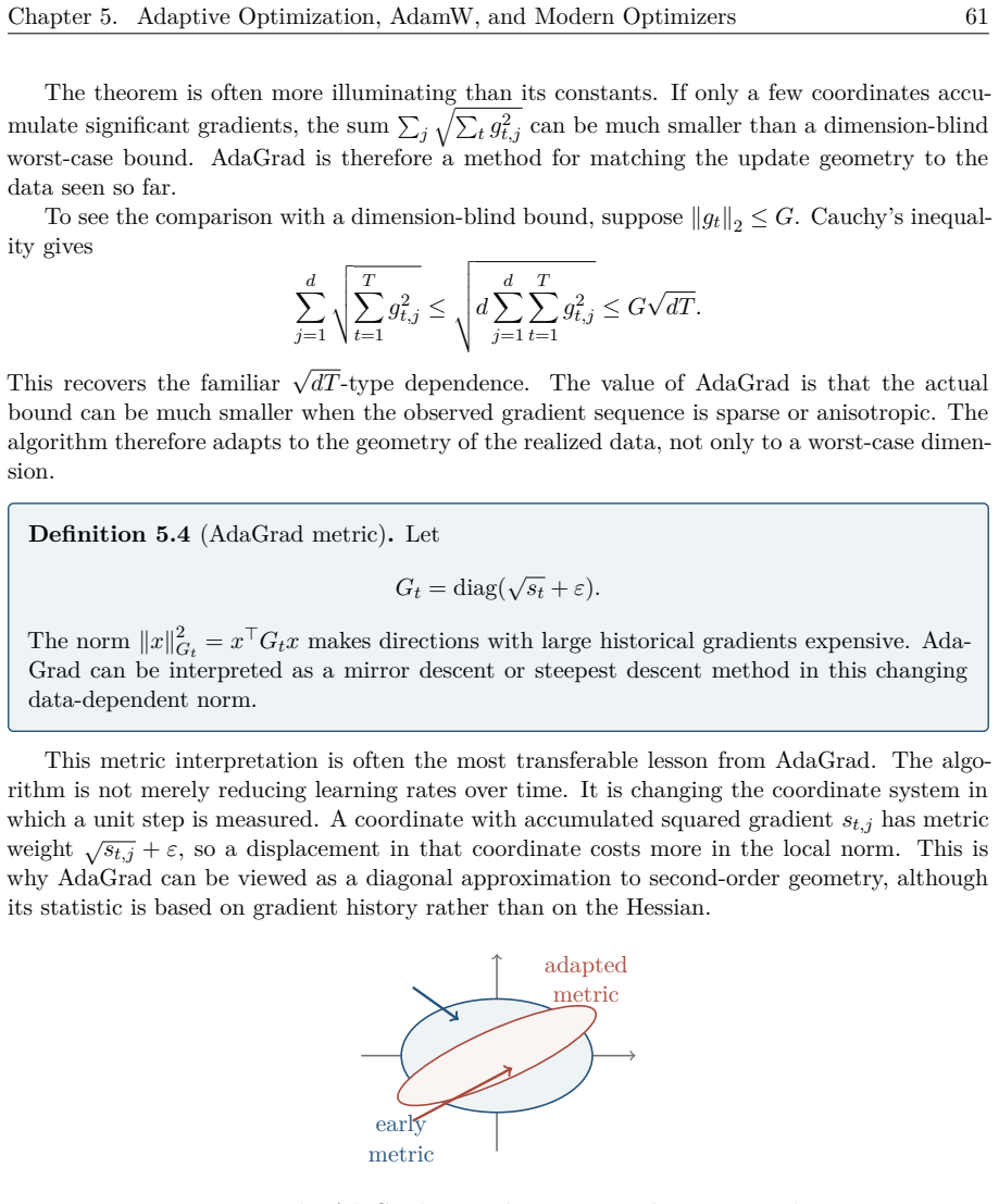
Figure 5.4. Figure 5.4: Optimizer theory combines geometry, statistics, and systems constraints. 5.2 AdaGrad and Data-Dependent Geometry AdaGrad is the cleanest starting point because it has a simple online-learning interpretation. At round t, an algorithm chooses θt , observes a loss ℓt , …
Figure 5.5
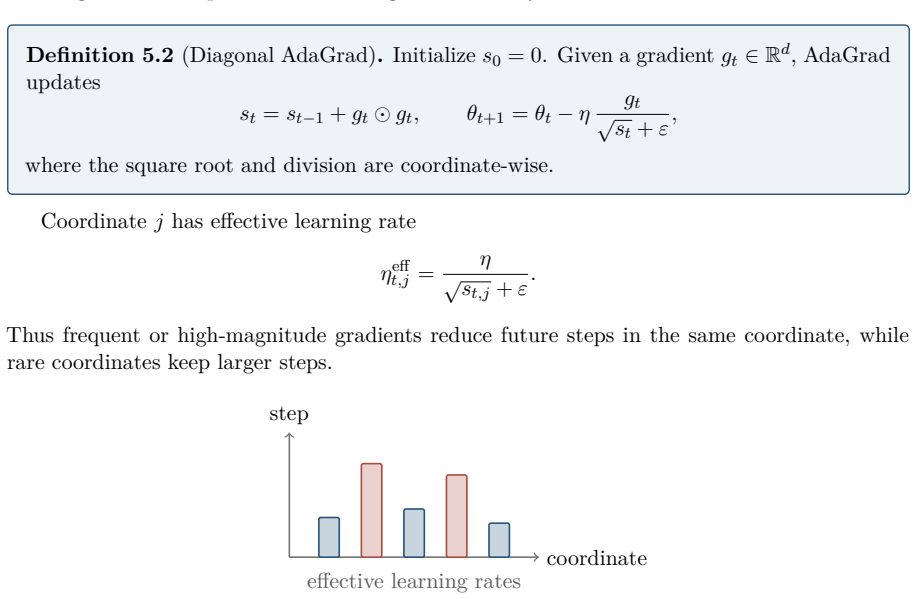
Figure 5.5. Figure 5.5: Adaptive methods use gradient history to choose later coordinate scales. Definition 5.2 (Diagonal AdaGrad). Initialize s0 = 0. Given a gradient gt ∈ R d , AdaGrad updates st = st−1 + gt gt , θt+1 = θt − η gt √ st + ε , where the square root and division are coordinat…
Figure 5.6
Figure 5.6. Figure 5.6: AdaGrad assigns different effective step sizes to different coordinates. Theorem 5.3 (AdaGrad coordinate-form regret bound). For convex G∞-Lipschitz losses on a bounded domain of diameter D, diagonal AdaGrad satisfies a regret bound of the form RT (u) ≲ [PITH_FULL_I…
Figure 5.7
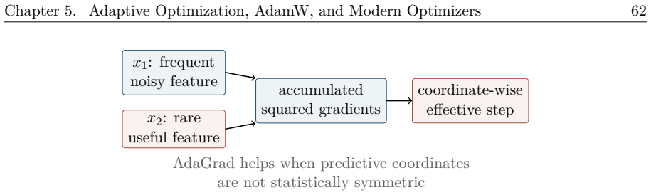
Figure 5.7. Figure 5.7: The AdaGrad norm changes as gradients accumulate. Example 5.5 (Rare but predictive features). Suppose x1 is a frequent noisy feature and x2 is a rare but predictive feature. A global learning rate treats their coordinates symmetrically. AdaGrad can reduce steps along…
Figure 5.8
Figure 5.8. Figure 5.8: Coordinate adaptivity is useful when the data distribution is anisotropic across features. AdaGrad also has limitations. Its classical regret theory is convex or online; deep networks are nonconvex. Diagonal scaling ignores correlations between parameters. The accumu…
Figure 5.9
Figure 5.9. Figure 5.9: Adam forgets old gradients exponentially, while AdaGrad keeps accumulating squared gradients. Definition 5.6 (Adam). Given parameters β1, β2 ∈ [0, 1), initialize m0 = v0 = 0. Adam [PITH_FULL_IMAGE:figures/full_fig_p071_5_9.png]
Figure 5.10
Figure 5.10. Figure 5.10: Adam’s coordinate-wise effective learning rate is inversely related to the estimated RMS scale. For coordinate j, η eff t,j = η p vbt,j + ε . Flat or low-gradient coordinates can receive larger steps; high-variance coordinates receive smaller steps. This normalizati…
Figure 5.11
Figure 5.11. Figure 5.11: AMSGrad repairs Adam’s convergence issue by using a monotone second-moment denominator. Definition 5.8 (AMSGrad). AMSGrad modifies Adam by setting vet = max(vet−1, vbt), θt+1 = θt − η mb t √ vet + ε , where the maximum is coordinate-wise. AMSGrad is important theore…
Figure 5.12
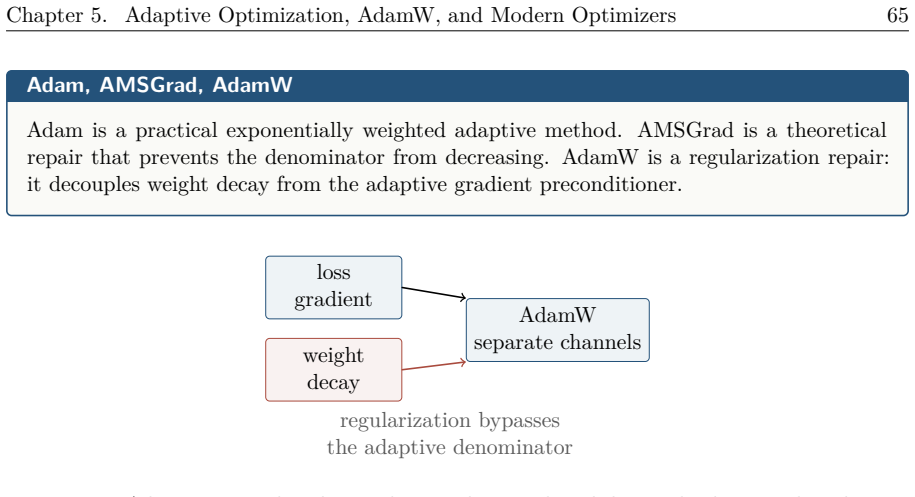
Figure 5.12. Figure 5.12: AdamW treats the adaptive loss-gradient path and the weight-decay path as distinct operations. 5.4 Implicit Bias and Generalization In overparameterized learning, many parameter vectors can interpolate the training data. The optimizer selects a path to one of them. …
Figure 5.13
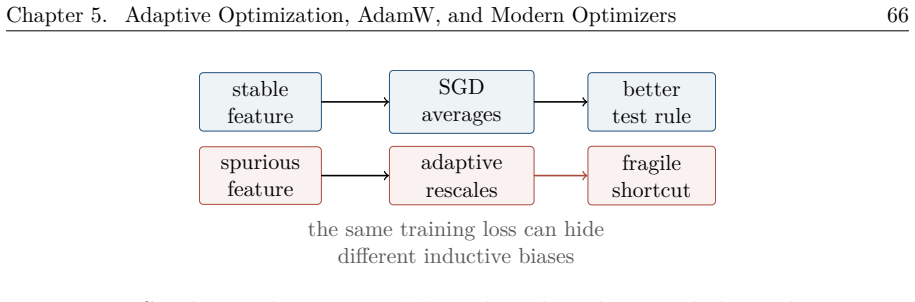
Figure 5.13. Figure 5.13: Different optimizers can reach different interpolating solutions from the same initialization. Proposition 5.10 (Marginal value phenomenon, informal). There are learning problems where adaptive gradient methods reach zero training error but converge to a classifier …
Figure 5.14
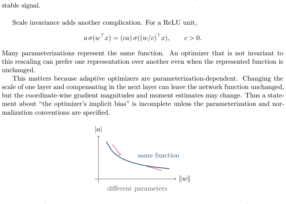
Figure 5.14. Figure 5.14: Coordinate adaptivity can help or hurt depending on which coordinates carry stable signal. Scale invariance adds another complication. For a ReLU unit, a σ(w >x) = (ca) σ((w/c) >x), c > 0. Many parameterizations represent the same function. An optimizer that is not …
Figure 5.15
Figure 5.15. Figure 5.15: Scale-equivalent parameterizations can represent the same ReLU function but induce different optimizer behavior. Definition 5.11 (Gradient flow with a metric). For a time-dependent positive semidefinite matrix P(t), the continuous time analogue of preconditioned des…
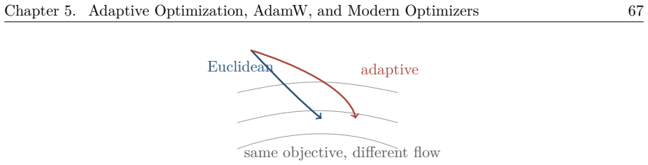
Figure 5.16
Figure 5.16. Figure 5.16: Changing the metric changes the continuous-time optimization flow. Once the training loss is nearly zero, the optimizer still matters because it determines the route to interpolation. SGD has noise-induced and geometry-induced biases; AdaGrad and Adam introduce coor…
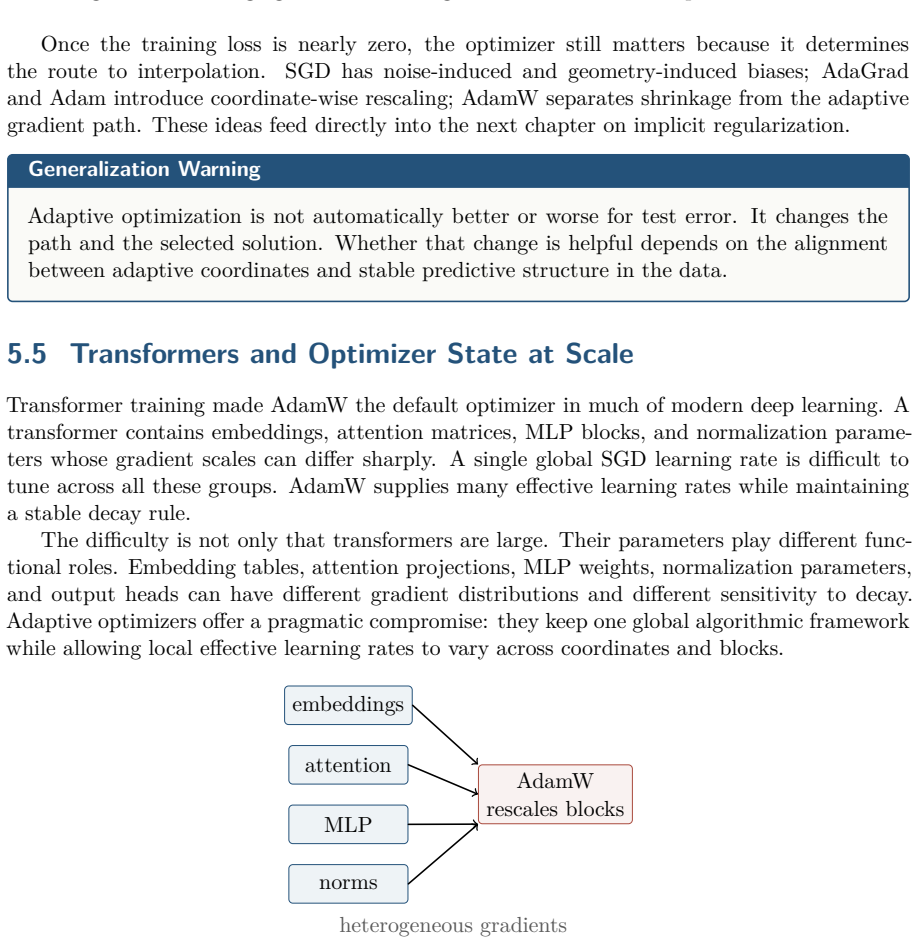
Figure 5.17
Figure 5.17. Figure 5.17: Transformer parameter groups naturally produce heterogeneous gradient scales. The same adaptivity that helps tuning also increases memory. For N parameters, Adam￾style training stores the parameters, gradients, first moments, and second moments, plus mixed￾precision…
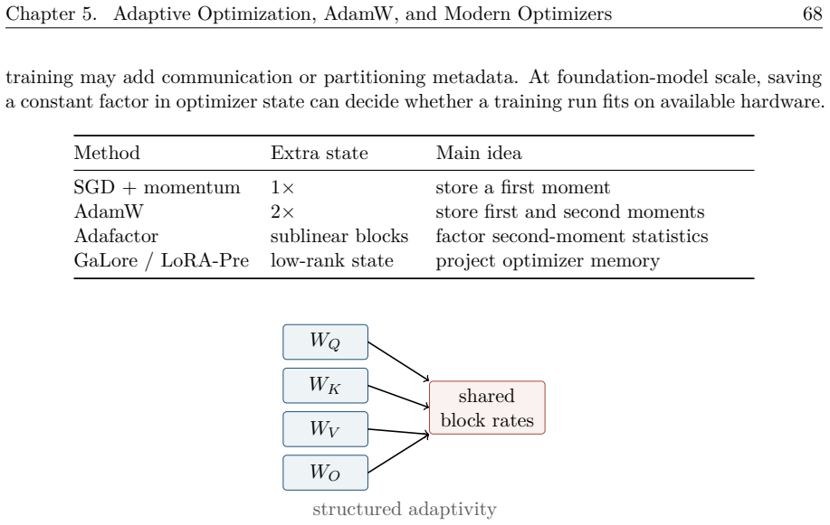
Figure 5.18
Figure 5.18. Figure 5.18: Adam-mini-style methods reduce the number of distinct effective learning-rate statistics by sharing rates within structured blocks. Remark 5.12 (Adam-mini). Adam-mini is motivated by the observation that many coor￾dinates in a large language model may not need separ…
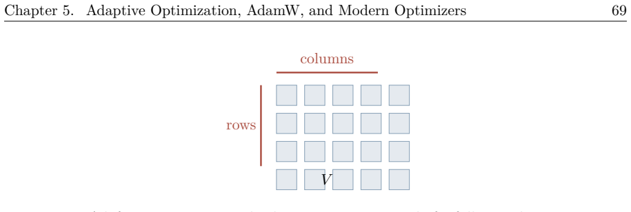
Figure 5.19
Figure 5.19. Figure 5.19: Adafactor stores row and column statistics instead of a full second-moment tensor for matrix parameters. Another route is to reduce the optimizer state by projecting gradients onto low-dimensional subspaces. Low-rank optimizer-state methods make a different assumpti…
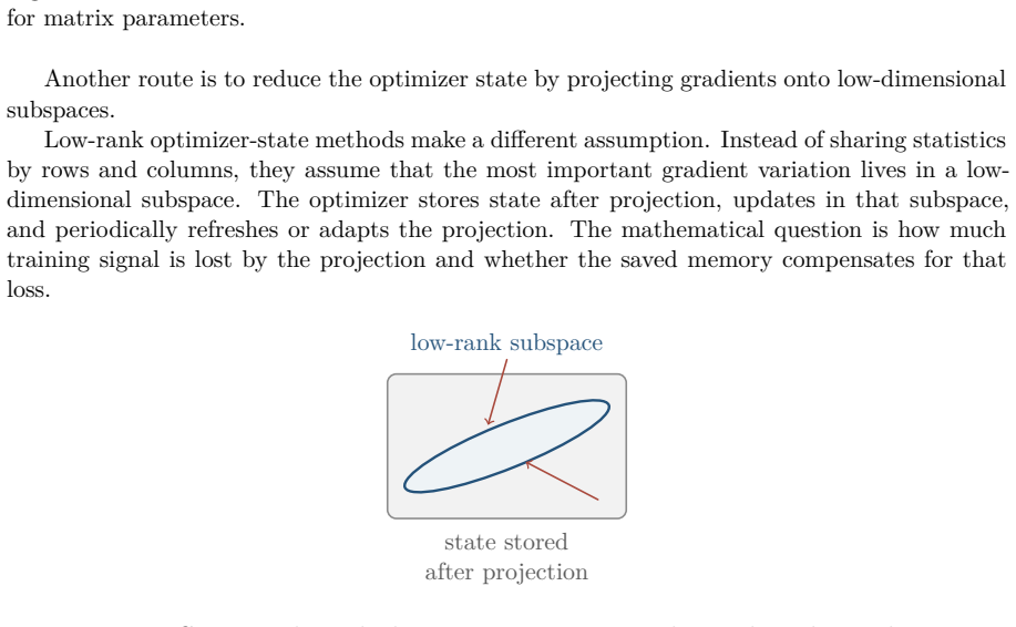
Figure 5.20
Figure 5.20. Figure 5.20: GaLore-style methods store optimizer state in low-rank gradient subspaces. 5.6 Modern Optimizer Frontier Modern optimizer work revisits the same questions under large-model constraints. How much curvature can be exploited cheaply? How much optimizer state is necessa…
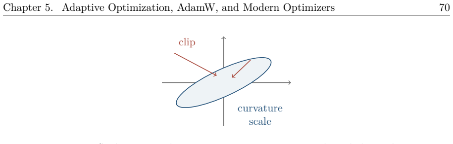
Figure 5.21
Figure 5.21. Figure 5.21: Sophia uses a cheap curvature estimate to rescale and clip updates. Remark 5.14 (Sophia). Sophia, or Second-order Clipped Stochastic Optimization, uses a lightweight diagonal Hessian or curvature estimate. Its goal is not full Newton training; it is to capture enoug…
Figure 5.22
Figure 5.22. Figure 5.22: Sign-momentum methods preserve coarse direction while discarding some magni￾tude information. Learning-rate schedules are another major part of modern training. A schedule-free opti￾mizer attempts to make schedule behavior internal to the algorithmic state. This doe…
Figure 5.23
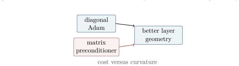
Figure 5.23. Figure 5.23: Schedule-free methods aim to reduce dependence on hand-designed decay curves. diagonal Adam matrix preconditioner better layer geometry cost versus curvature [PITH_FULL_IMAGE:figures/full_fig_p080_5_23.png]
Figure 5.24
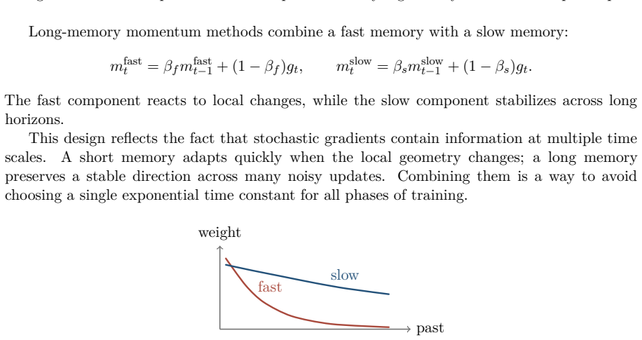
Figure 5.24. Figure 5.24: Matrix preconditioners exploit richer layer geometry but cost more per step. Long-memory momentum methods combine a fast memory with a slow memory: mfast t = βfmfast t−1 + (1 − βf )gt , mslow t = βsmslow t−1 + (1 − βs)gt . The fast component reacts to local changes,…
Figure 5.25
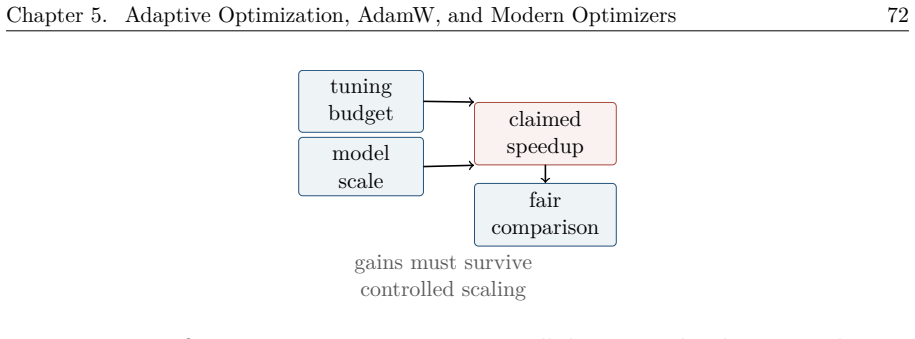
Figure 5.25. Figure 5.25: AdEMAMix-style methods combine short and long momentum memories. Finally, benchmarking optimizers is hard. A new optimizer may win because it received more tuning, because a small-scale proxy did not reflect large-scale behavior, or because wall-clock time, tokens, …
Figure 5.26
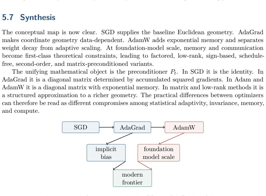
Figure 5.26. Figure 5.26: Optimizer comparisons require controlled tuning and scaling protocols. 5.7 Synthesis The conceptual map is now clear. SGD supplies the baseline Euclidean geometry. AdaGrad makes coordinate geometry data-dependent. AdamW adds exponential memory and separates weight d…
Figure 5.27
Figure 5.27. Figure 5.27: The optimizer frontier extends the SGD-to-AdaGrad-to-AdamW story under implicit-bias and scale constraints. Remark 5.15 (Key takeaways). First, adaptivity chooses a geometry: AdaGrad and Adam are data-dependent preconditioners, not merely faster SGD variants. Second…
Figure 6.1
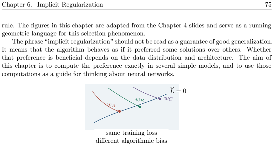
Figure 6.1. Figure 6.1: Interpolation leaves a set of zero-error solutions. The optimizer and its parameteri￾zation select a particular point on this set. The chapter develops a three-step story. A parameterization w = g(θ) changes the coordi￾nates in which gradient descent is run. Those co…
Figure 6.2
Figure 6.2. Figure 6.2: The chapter’s organizing principle: coordinates induce geometry, and geometry determines the implicit bias of the path. 6.2 The Running Least-Squares Model The cleanest model in which to see implicit regularization is an underdetermined least-squares problem. Let f(x…
Figure 6.3
Figure 6.3. Figure 6.3: The minimum-norm interpolant is the point where the affine solution set meets the row space. Other feasible points differ by null-space directions. Lemma 6.2 (Minimum-norm bias of gradient flow). Assume Ax = b is consistent. Let x(0) = 0 and x˙(t) = −A >(Ax(t) − b). …
Figure 6.4
Figure 6.4. Figure 6.4: Vanishing ridge regularization is an explicit proxy for the implicit ℓ2 bias of direct gradient flow from the origin. 6.3 Reparameterization Changes the Bias Now reparameterize the same least-squares problem by the entrywise square map x = sq(y) = y 2 , bf(y) = 1 2 …
Figure 6.5
Figure 6.5. Figure 6.5: Different norms select different feasible points. The corners of the ℓ1 ball explain why ℓ1 minimization promotes sparsity [PITH_FULL_IMAGE:figures/full_fig_p088_6_5.png]
Figure 6.6
Figure 6.6. Figure 6.6: A sparse signal has a small number of large coordinates. Basis pursuit uses ℓ1 geometry to find such feasible points. Example 6.7 (A two-dimensional toy problem). Let A = h 1 2i , b = 1, x ≥ 0. The feasible set is the line segment x1 + 2x2 = 1. Direct computation giv…
Figure 6.7
Figure 6.7. Figure 6.7: In the toy problem, the ℓ2 and nonnegative ℓ1 selected solutions are different points on the same feasible line segment [PITH_FULL_IMAGE:figures/full_fig_p089_6_7.png]
Figure 6.8
Figure 6.8. Figure 6.8: Gradient descent minimizes a linearized objective plus a quadratic penalty on the step length. Definition 6.8 (Bregman divergence). Let ϕ : R m → R be differentiable and strictly convex on a convex domain. The Bregman divergence generated by ϕ is Dϕ(x, z) = ϕ(x) − ϕ(…
Figure 6.9
Figure 6.9. Figure 6.9: Bregman divergence measures the vertical gap between a convex function and its tangent approximation [PITH_FULL_IMAGE:figures/full_fig_p090_6_9.png]
Figure 6.10
Figure 6.10. Figure 6.10: At the Bregman projection, the gradient of the divergence is normal to the feasible affine set. 6.5.1 Square Flow as Entropy Mirror Flow For the entropy mirror map, ∇2ϕ(x) = D−1 x . The continuous-time mirror flow associated with f is x˙(t) = −(∇2ϕ(x(t)))−1∇f(x(t)).…
Figure 6.11
Figure 6.11. Figure 6.11: Putting the pieces together: square parameterization induces entropy mirror ge￾ometry, whose small-initialization KL projection converges to ℓ1 selection. 6.6 Connections to Deep Learning Neural networks are highly reparameterized models. Layers can be scaled agains…
Figure 6.12
Figure 6.12. Figure 6.12: Neural networks can interpolate in many parameter configurations. Implicit bias asks which configuration and which predictor the training path selects. 6.6.1 Linear Classification and Maximum Margin A second canonical example concerns separable linear classification…
Figure 6.13
Figure 6.13. Figure 6.13: The maximum-margin separator classifies the training data correctly and maxi￾mizes the normalized distance to the closest examples. The reference notes also mention the generalization-bound motivation: classical margin bounds for support vector machines suggest that…
Figure 7.1
Figure 7.1. Figure 7.1: Generalization compares the error measured on the finite training sample with the error under the distribution that produced the sample. Definition 7.1 (Empirical and population error). Let S = {(xi , yi)} N i=1 be drawn inde￾pendently from a distribution D on R d × …
Figure 7.2
Figure 7.2. Figure 7.2: Three views of capacity. Finite-class bounds count hypotheses, VC theory counts labelings on finite samples, and data-dependent bounds measure the hypotheses that matter on the observed distribution. 7.2 Finite Hypothesis Classes The cleanest result is obtained when …
Figure 7.3
Figure 7.3. Figure 7.3: The finite-class proof is Hoeffding for one hypothesis followed by a union bound over the bad events Bh. The theorem is agnostic: it makes no assumption that the labels are generated by a member of H. Under a realizability assumption one can obtain a faster 1/N depen…
Figure 7.4
Figure 7.4. Figure 7.4: Finite-class bounds can be read as an Occam principle: short descriptions that fit many examples are statistically meaningful. Remark 7.5. The factor log |H| is the description cost of selecting one member of the class. This is too crude for real-valued neural networ…
Figure 7.5
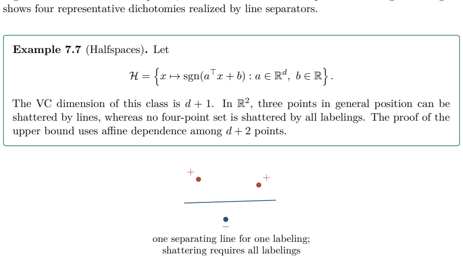
Figure 7.5. Figure 7.5: To shatter three points, a class must realize all 2 3 possible labelings. The figure shows four representative dichotomies realized by line separators. Example 7.7 (Halfspaces). Let H = n x 7→ sgn(a >x + b) : a ∈ R d , b ∈ R o . The VC dimension of this class is d + …
Figure 7.6
Figure 7.6. Figure 7.6: A single successful separation is not shattering. Shattering is a uniform statement over every assignment of labels to the same points. One must also be careful not to confuse VC dimension with parameter count. The class H = {x 7→ sgn(sin(ax)) : a ∈ R} has only one r…
Figure 7.7
Figure 7.7. Figure 7.7: Parameter count alone does not determine capacity. The geometry of the function family matters. Lemma 7.9 (Sauer–Shelah lemma). If VCdim(H) = k, then for every N, GH(N) ≤ X k i=0 N i ! . In particular, when N > k, GH(N) ≤  eN k k . The significance of the Sauer–She…
Figure 7.8
Figure 7.8. Figure 7.8: The ghost-sample argument replaces population error by an independent sample, and Rademacher signs randomize which point in each pair belongs to which sample. 7.4 VC Bounds for Neural Networks We now return to neural networks. To keep the combinatorics transparent, t…
Figure 7.9
Figure 7.9. Figure 7.9: A sign network is a composition of vector-valued layers. The proof counts label patterns neuron by neuron and layer by layer. Lemma 7.12 (Product rule for growth functions). Let H1 ⊆ YX 1 and H2 ⊆ YX 2 . For the product class H = H1 × H2, meaning x 7→ (h1(x), h2(x)),…
Figure 7.10
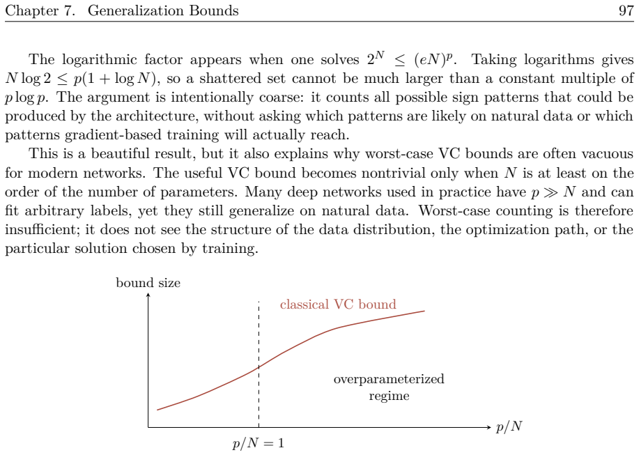
Figure 7.10. Figure 7.10: The classical parameter-counting bound becomes vacuous when the number of parameters substantially exceeds the number of examples. 7.5 PAC Learnability VC dimension is not merely a proof technique for a convenient bound. In the distribution-free realizable setting, …
Figure 7.11
Figure 7.11. Figure 7.11: If a large support is shattered, arbitrary labels on unseen points remain possible after observing only part of the support. Remark 7.16 (Agnostic PAC learning). The same characterization extends to the noisy, agnostic setting: a concept class is agnostically PAC le…
Figure 7.12
Figure 7.12. Figure 7.12: Rademacher complexity labels the sample with random signs and asks for the best correlation achievable by hypotheses in the class. 7.6.1 Random labels and deep networks A tempting hope is that although a deep network has large VC dimension, the combination of natura…
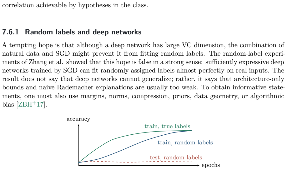
Figure 7.13
Figure 7.13. Figure 7.13: Deep networks can eventually fit random labels, while test accuracy under random labels remains at chance. Expressivity alone is not a generalization explanation. 7.7 Margins, Fat Shattering, and PAC-Bayes The last part of the chapter surveys two ways to describe a …
Figure 7.14
Figure 7.14. Figure 7.14: Occam’s principle reappears in several forms: finite-class indices, growth-function label patterns, and PAC-Bayes KL divergence. 7.8 What the Bounds Explain, and What They Do Not Classical generalization theory explains several fundamental facts. It shows why finite…
Figure 7.15
Figure 7.15. Figure 7.15: Small population error is not explained by training fit alone. The useful theory must also describe capacity, data structure, and algorithmic selection. The conceptual endpoint of the chapter is therefore not that VC theory is wrong. On the contrary, finite VC dimen…
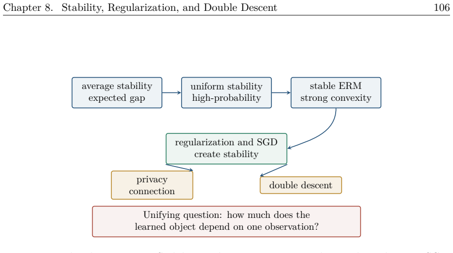
Figure 8.1
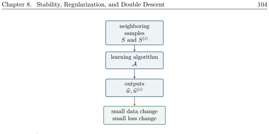
Figure 8.1. Figure 8.1: Stability is an algorithmic notion: neighboring samples should lead to nearby out￾puts, or at least to similar losses on test points. Definition 8.1 (Risk, empirical risk, and generalization error). Let z = (x, y) ∼ D, and let S = (z1, . . . , zN ) ∼ DN be an iid tra…
Figure 8.2
Figure 8.2. Figure 8.2: The generalization gap compares the population risk with the empirical risk at the learned output [PITH_FULL_IMAGE:figures/full_fig_p113_8_2.png]
Figure 8.3
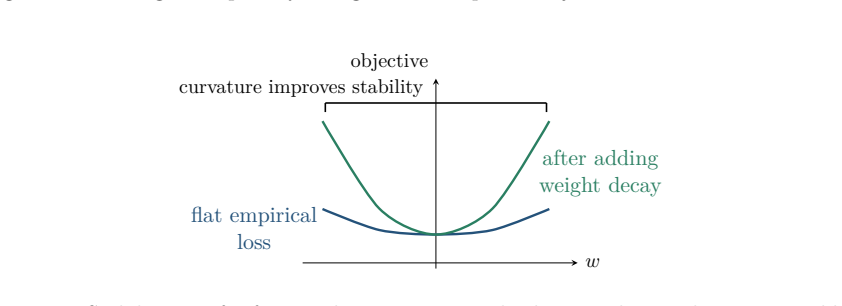
Figure 8.3. Figure 8.3: Adding an ℓ2 penalty changes a flat empirical objective into a more curved one. w objective flat empirical loss after adding weight decay curvature improves stability [PITH_FULL_IMAGE:figures/full_fig_p114_8_3.png]
Figure 8.4
Figure 8.4. Figure 8.4: Stability proofs often need curvature. Weight decay is the simplest way to add it. 8.2 Average Stability The stability viewpoint treats a learning algorithm as a map A : Z N → Ω, S 7→ A(S). For randomized algorithms, the map also depends on internal randomness, and e…
Figure 8.5
Figure 8.5. Figure 8.5: The chapter map. Stability is the organizing principle; regularized ERM, SGD, privacy, and double descent provide different views of it. S A wb = A(S) [PITH_FULL_IMAGE:figures/full_fig_p115_8_5.png]
Figure 8.6
Figure 8.6. Figure 8.6: A learning algorithm is a sample-dependent map from datasets to parameters. S : S ′ : S (i) : z1 z2 · · · zi · · · zN z ′ 1 z ′ 2 · · · z ′ i · · · z ′ N z1 z2 · · · z ′ i · · · zN replace only i [PITH_FULL_IMAGE:figures/full_fig_p115_8_6.png]
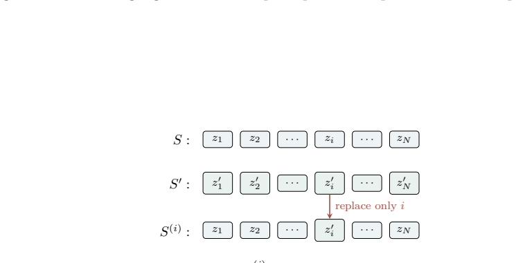
Figure 8.7
Figure 8.7. Figure 8.7: The hybrid sample S (i) differs from S in exactly one coordinate [PITH_FULL_IMAGE:figures/full_fig_p115_8_7.png]
Figure 8.8
Figure 8.8. Figure 8.8: Uniform stability is stronger than average stability and leads to more direct high￾probability control. We write ∆unif(A) ≤ γ. This is a worst-case condition over the sample, the replaced coordinate, and the test point. The handwritten notes use the equivalent chapte…
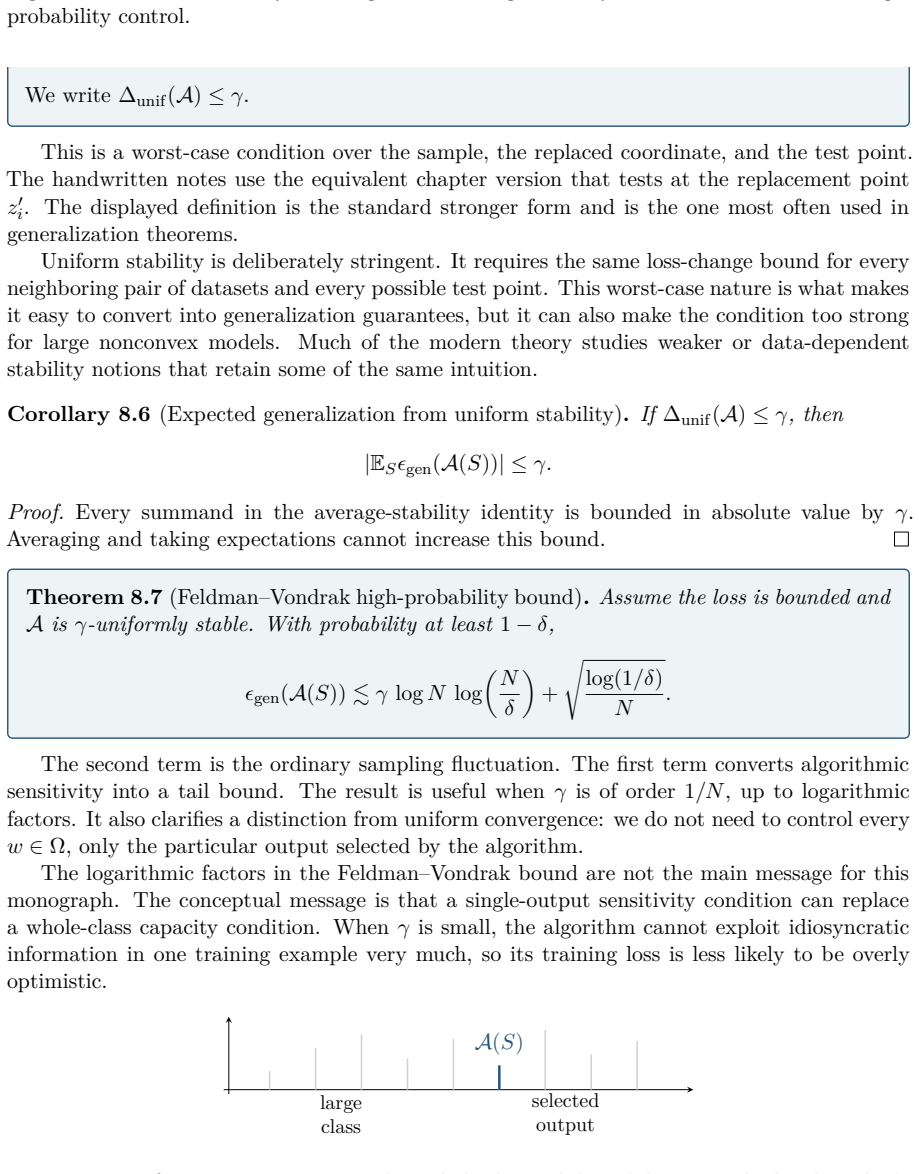
Figure 8.9
Figure 8.9. Figure 8.9: Uniform convergence controls a whole class, while stability controls the algorithm’s selected output under a neighboring-sample perturbation [PITH_FULL_IMAGE:figures/full_fig_p117_8_9.png]
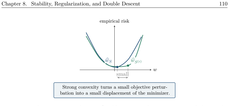
Figure 8.10
Figure 8.10. Figure 8.10: The geometric mechanism of stable ERM. Replacing one summand changes the objective only slightly; curvature prevents the minimizer from moving far. Proof sketch of the ERM stability theorem. By the lemma, the empirical risk RS is α-strongly convex. Since wbS minimiz…
Figure 8.11
Figure 8.11. Figure 8.11: The stable-ERM proof has two steps: curvature gives nearby minimizers, and Lipschitzness turns nearby minimizers into nearby losses. 8.5 Regularization, SGD, and Privacy 8.5.1 Explicit regularization When the original loss is convex but not strongly convex, one can …
Figure 8.12
Figure 8.12. Figure 8.12: Choosing the regularization strength balances stability and bias. 8.5.2 Implicit regularization by SGD Stochastic gradient descent can also be stable without an explicit quadratic penalty. The reason is dynamic: two coupled runs on neighboring samples see the same e…
Figure 8.13
Figure 8.13. Figure 8.13: The SGD coupling proof runs the two algorithms with the same sampled indices. Most steps are shared; only hits to the replaced example create drift. Definition 8.13 (Expected uniform stability). For a randomized algorithm, one common stability notion is sup S,S(i) ,…
Figure 8.14
Figure 8.14. Figure 8.14: Stability and privacy are both single-sample sensitivity notions, but they control different objects. 8.6 Double Descent The classical bias–variance story says that as model capacity increases, bias decreases while variance increases, leading to a U-shaped test-erro…
Figure 8.15
Figure 8.15. Figure 8.15: The modern double-descent curve augments the classical U-shaped picture with an overparameterized branch after interpolation. Proposition 8.16 (Squared-error bias–variance decomposition). Let y = f(x) + ε, E[ε | x] = 0, Var(ε | x) = σ 2 , [PITH_FULL_IMAGE:figures/f…
Figure 8.16
Figure 8.16. Figure 8.16: In overparameterized linear regression, many interpolators may fit the data. Gra￾dient descent from near zero selects the minimum-norm solution. Definition 8.17 (Minimum-norm least-squares estimator). Consider yi = x > i β + εi , xi ∈ R p , i = 1, . . . , n, and let…
Figure 8.17
Figure 8.17. Figure 8.17: A schematic reading of the ridgeless-risk formula. The risk spikes near p/n = 1; beyond interpolation it may decrease depending on the signal-to-noise ratio. Let SNR = r 2/σ2 . The null predictor bβ = 0 has risk r 2 , and as γ → ∞ the ridgeless risk approaches this …
Figure 8.18
Figure 8.18. Figure 8.18: Linear ridgeless regression is a solvable model of a phenomenon that also appears in overparameterized neural networks: interpolation need not imply poor test performance [PITH_FULL_IMAGE:figures/full_fig_p124_8_18.png]
Figure 9.1
Figure 9.1. Figure 9.1: The chapter moves from exact ridgeless-risk formulas to computational lower bounds for nonlinear classes related to neural networks. approximation representation optimization training generalization test error computation efficiency deep learning theory [PITH_FULL_I…
Figure 9.2
Figure 9.2. Figure 9.2: Four lenses on a learning problem. This chapter completes a statistical-risk story and then focuses on efficient learnability [PITH_FULL_IMAGE:figures/full_fig_p127_9_2.png]
Figure 9.3
Figure 9.3. Figure 9.3: A schematic double-descent curve. Interpolation changes the classical bias–variance picture by creating a high-risk threshold and a possible second descent. The first part of the chapter asks where this curve comes from in a solvable model. The second part asks a dif…
Figure 9.4
Figure 9.4. Figure 9.4: When p > n, many directions are invisible to the rows of X. The conditional bias is the prediction norm of the nullspace component Πβ. 9.2.1 Isotropic Gaussian Designs The formulas become explicit for isotropic Gaussian features. Suppose xi ∼ N(0, Ip), Σ = Ip, γ = p …
Figure 9.5
Figure 9.5. Figure 9.5: A schematic Marchenko–Pastur density in an underparameterized regime. The inverse moment controls the variance. eigenvalue density zero mass γ > 1 [PITH_FULL_IMAGE:figures/full_fig_p131_9_5.png]
Figure 9.6
Figure 9.6. Figure 9.6: In the overparameterized regime, Σb has a nullspace. The pseudoinverse ignores the zero eigenvalues but the nonzero spectrum still determines the variance. packages the inverse moments of the sample spectrum. Closed forms for this transform under Marchenko–Pastur asy…
Figure 9.7
Figure 9.7. Figure 9.7: Ridgeless double descent arises from two terms: variance from the inverse sample spectrum and bias from the signal in the nullspace. This section uses the language of PAC learning. The emphasis is not on sharp sample￾complexity constants, but on the distinction betwe…
Figure 9.8
Figure 9.8. Figure 9.8: A lower bound can depend on statistical resources, computational resources, and restrictions on the learner’s output class. Theorem 9.4 (Blum–Rivest, informal). For a depth-two threshold network with three com￾putational nodes, deciding whether some choice of weights…
Figure 9.9
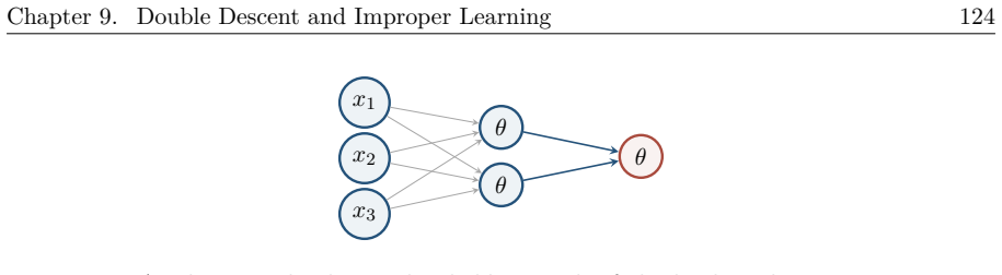
Figure 9.9. Figure 9.9: A schematic depth-two threshold network of the kind used to motivate proper￾training hardness. For a target class H, the benchmark error is OPTH = inf h∈H errD(h). A learner competes with H if, with high probability over the sample and its internal ran￾domness, it re…
Figure 9.10
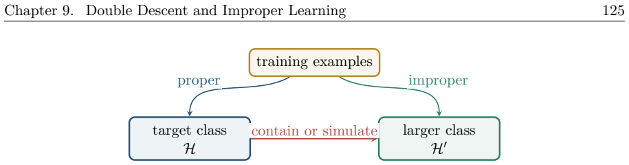
Figure 9.10. Figure 9.10: Improper learning is an escape hatch: output a different kind of predictor while still competing with the original class. representation if that representation supports a simple algorithm. Definition 9.7 (CNF and DNF classes). A 3-CNF formula is a conjunction of cla…
Figure 9.11
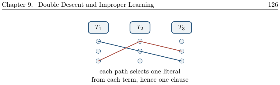
Figure 9.11. Figure 9.11: The CNF obtained from a three-term DNF is highly structured: every clause chooses one literal from each original term. Theorem 9.10 (Valiant-style improper learning, informal). For constant k, a k-term DNF can be learned in polynomial time by outputting a hypothesis…
Figure 9.12
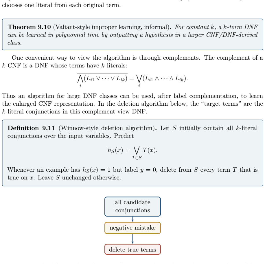
Figure 9.12. Figure 9.12: The deletion algorithm starts from a very large class and removes only candidates contradicted by negative examples. Lemma 9.12 (No false deletions). Suppose a conjunction T is one of the terms in the target DNF being learned in the complement view. The deletion alg…
Figure 9.13
Figure 9.13. Figure 9.13: Improper learning enlarges the output class. This may make the algorithm easy while increasing the number of samples needed for uniform generalization. 9.5 Neural Networks, Halfspaces, and Cryptographic Hardness The DNF example prevents a common mistake: proper hard…
Figure 9.14
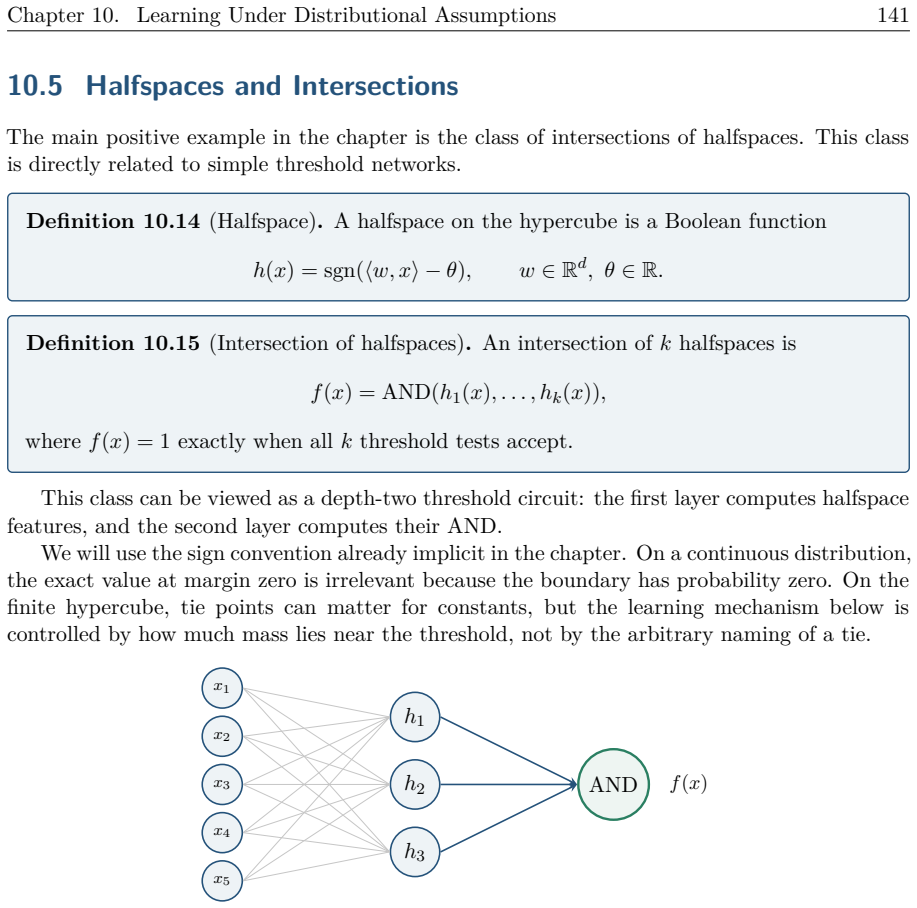
Figure 9.14. Figure 9.14: Intersections of halfspaces carve out regions by requiring several linear threshold tests to be simultaneously satisfied. Threshold activations are halfspace tests. If hidden units output gj (x) ∈ {−1, +1}, then the AND of m such tests can be written as a single thr…
Figure 9.15
Figure 9.15. Figure 9.15: An intersection of halfspaces can be implemented by a depth-two threshold network: hidden nodes compute halfspaces and the output node computes their AND. the output class does not remove the computational barrier under the assumed hardness of the underlying lattice…
Figure 9.16
Figure 9.16. Figure 9.16: A lattice is a discrete set closed under integer linear combinations. The crypto￾graphic hardness result uses assumptions related to approximating short lattice vectors. The reduction idea follows a standard cryptographic template. In a public-key encryption system,…
Figure 9.17
Figure 9.17. Figure 9.17: If the decryption function were efficiently learnable, chosen-message examples would train an attacker to predict decryptions of fresh ciphertexts. Remark 9.18. The hard distribution in this theorem is not a natural image or language distribution. It is produced by …
Figure 9.18
Figure 9.18. Figure 9.18: A computational–statistical tradeoff. Enlarging the output class can reduce search difficulty while increasing the sample complexity required to control generalization. Proper hardness can disappear under improper learning, as the DNF example shows. Cryp￾tographic h…
Figure 10.1
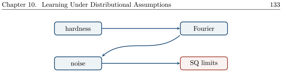
Figure 10.1. Figure 10.1: The chapter’s roadmap: distributional assumptions expose Fourier structure; noise sensitivity certifies concentration; and parity functions show where statistical-query methods break down. arbitrary distribution uniform hypercube Gaussian space assumptions invarianc…
Figure 10.2
Figure 10.2. Figure 10.2: A structured distribution is not a cosmetic assumption. It changes which statistics are informative and which algorithms become plausible. parity functions hide all of their mass in a single high-degree coefficient, making them almost invisible to algorithms that on…
Figure 10.3
Figure 10.3. Figure 10.3: The chapter’s dictionary: boundary geometry, noise stability, Fourier concentration, algorithms, and lower bounds are different views of the same structure. 10.2 Fourier Analysis on the Hypercube We work first on the Boolean hypercube {±1} d = {−1, +1} d with the un…
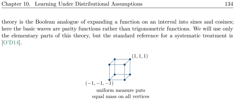
Figure 10.4
Figure 10.4. Figure 10.4: The Boolean hypercube. The uniform distribution gives every vertex the same probability, making orthogonality calculations exact. The hypercube has a natural orthonormal basis indexed by subsets of coordinates. Definition 10.1 (Parity characters). For S ⊆ [d], the p…
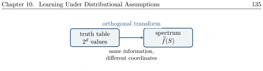
Figure 10.5
Figure 10.5. Figure 10.5: The Fourier transform on the hypercube rewrites the truth table in an orthonormal coordinate system. j ∈ S4T. Independence and E[xj ] = 0 give Ex[χS(x)χT (x)] = Ex[χS4T (x)] = E[xj ] Y i∈S4T, i6=j E[xi ] = 0. When S = T, the product is identically 1. The coefficient…
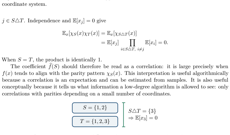
Figure 10.6
Figure 10.6. Figure 10.6: A nonempty symmetric difference leaves at least one independent mean-zero sign, which kills the inner product. Theorem 10.4 (Parseval identity). For every f : {±1} d → R, Ex[f(x) 2 ] = X S⊆[d] bf(S) 2 . In particular, if f(x) ∈ {±1}, then P S bf(S) 2 = 1. Proof. Exp…
Figure 10.7
Figure 10.7. Figure 10.7: Low-degree truncation keeps the Fourier mass below a degree cutoff and discards the high-degree tail. 10.3 Low-Degree Learning Definition 10.6 (Fourier concentration). A function f : {±1} d → R is α(ϵ, d)-concentrated if X |S|≥α(ϵ,d) bf(S) 2 ≤ ϵ. A concept class H i…
Figure 10.8
Figure 10.8. Figure 10.8: The low-degree algorithm estimates the relevant correlations and assembles them into a polynomial classifier. More concretely, for every S ⊆ [d] with |S| < α, the learner estimates gb(S) = 1 m Xm i=1 yiχS(xi). It then forms g(x) = X |S|<α gb(S)χS(x), h(x) = sgn(g(x)…
Figure 10.9
Figure 10.9. Figure 10.9: For a new class, the algorithmic part is generic. The mathematical work is to prove a structural concentration theorem. The remainder of the positive part of the chapter explains one powerful way to prove con￾centration: show that the function is stable under random…
Figure 10.10
Figure 10.10. Figure 10.10: The noise operator flips coordinates independently. A function is noise stable if these local perturbations rarely change the label. Noise sensitivity has an exact Fourier formula. Proposition 10.11 (Spectral formula for noise sensitivity). For Boolean f : {±1} d →…
Figure 10.11
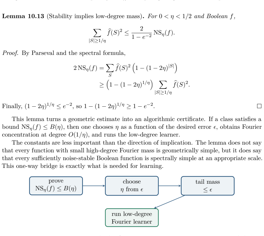
Figure 10.11. Figure 10.11: The noise multiplier (1 − 2η) k damps high-degree Fourier components first. Lemma 10.13 (Stability implies low-degree mass). For 0 < η < 1/2 and Boolean f, X |S|≥1/η bf(S) 2 ≤ 2 1 − e−2 NSη(f). Proof. By Parseval and the spectral formula, 2 NSη(f) = X S bf(S) 2  1…
Figure 10.12
Figure 10.12. Figure 10.12: Noise sensitivity is a bridge from geometry to Fourier concentration and then to an explicit learning algorithm [PITH_FULL_IMAGE:figures/full_fig_p149_10_12.png]
Figure 10.13
Figure 10.13. Figure 10.13: An intersection of halfspaces is a depth-two threshold architecture: hidden units compute linear threshold functions and the output gate computes their conjunction. Theorem 10.16 (Peres noise bound). For every halfspace h and every 0 < η < 1/2, NSη(h) ≤ C √ η for a…
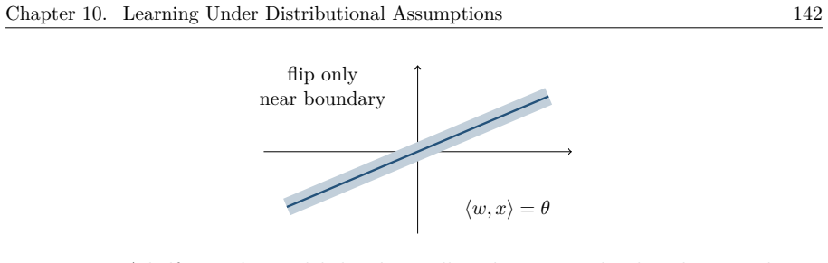
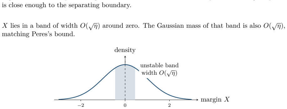
Figure 10.14
Figure 10.14. Figure 10.14: A halfspace changes label under small random noise only when the original point is close enough to the separating boundary. X lies in a band of width O( √η) around zero. The Gaussian mass of that band is also O( √η), matching Peres’s bound. margin X density −2 0 2 …
Figure 10.15
Figure 10.15. Figure 10.15: For majority, the normalized margin is approximately Gaussian. A sign change is likely only near the threshold. Noise stability is also compositional. Proposition 10.17 (Union bound for noise sensitivity). If h(x) = g(f1(x), . . . , fk(x)), then NSη(h) ≤ X k i=1 NS…
Figure 10.16
Figure 10.16. Figure 10.16: For Gaussian inputs, the span of the halfspace normals can be identified from distributional changes in labeled examples [PITH_FULL_IMAGE:figures/full_fig_p152_10_16.png]
Figure 10.17
Figure 10.17. Figure 10.17: Samples simulate statistical queries by empirical averaging. The model is powerful enough to include many moment, correlation, and gradient-based procedures. Population gradients in neural-network training, for instance, are expectations: ∇θL(θ) = E(x,y) [∇θℓ(fθ(x)…
Figure 10.18
Figure 10.18. Figure 10.18: SQ algorithms see stable aggregate information. They may miss exact combina￾torial structure present in the raw sample. Definition 10.22 (Unknown parity). Choose an unknown set T ⊆ [d]. Draw x ∼ Unif({±1} d ) and label y = χT (x) = Y i∈T xi . The Fourier spectrum o…
Figure 10.19
Figure 10.19. Figure 10.19: Raw parity samples give a linear system over F2. This exact combinatorial information is not available to an SQ learner. Noisy parity is different again. If each label is flipped independently with a constant probabil￾ity below 1/2, the exact linear-system trick be…
Figure 11.1
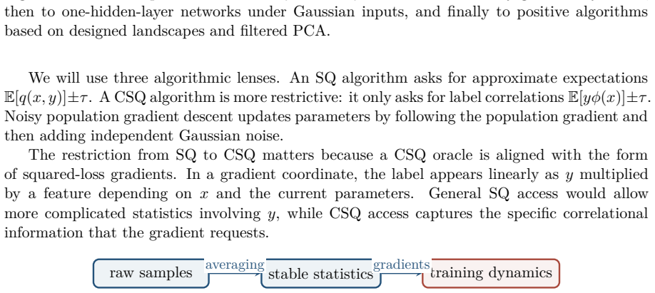
Figure 11.1. Figure 11.1: The chapter moves from SQ and CSQ lower bounds to noisy gradient dynamics, then to one-hidden-layer networks under Gaussian inputs, and finally to positive algorithms based on designed landscapes and filtered PCA. We will use three algorithmic lenses. An SQ algorith…
Figure 11.2
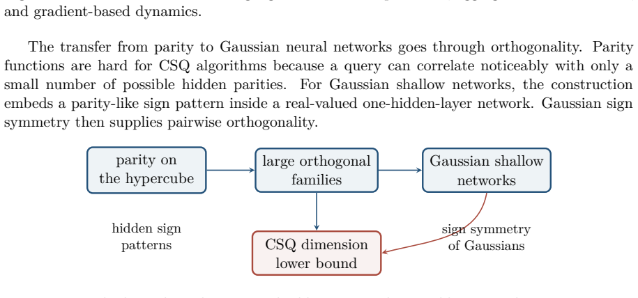
Figure 11.2. Figure 11.2: Three views of a learning algorithm: raw sample access, aggregate statistical access, and gradient-based dynamics. The transfer from parity to Gaussian neural networks goes through orthogonality. Parity functions are hard for CSQ algorithms because a query can corre…
Figure 11.3
Figure 11.3. Figure 11.3: The lower-bound strategy: build many nearly invisible targets by turning parity￾like sign patterns into Gaussian shallow-network functions [PITH_FULL_IMAGE:figures/full_fig_p158_11_3.png]
Figure 11.4
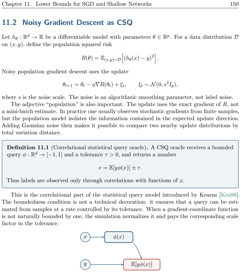
Figure 11.4. Figure 11.4: A CSQ sees the label only through a correlation with a chosen feature of the input. The connection to gradients is direct. Proposition 11.2 (Gradient coordinates are CSQs). Assume the marginal distribution of x is known and that the relevant gradient-coordinate func…
Figure 11.5
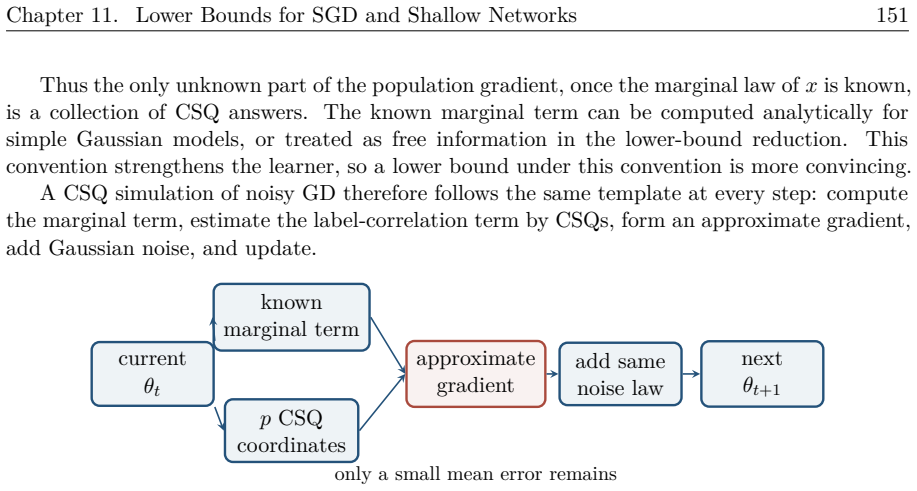
Figure 11.5. Figure 11.5: A CSQ algorithm can simulate the distribution of a noisy population GD step if the gradient estimate is accurate enough. The simulation is distributional rather than pointwise: we want the noisy update produced by the CSQ simulation to agree with the noisy GD update…
Figure 11.6
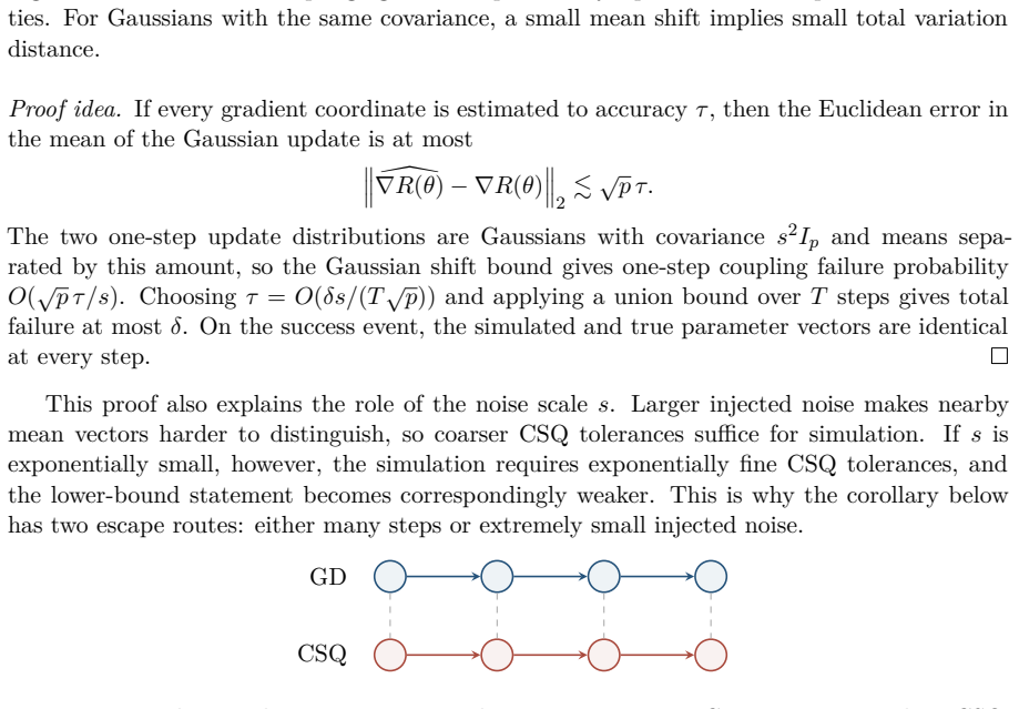
Figure 11.6. Figure 11.6: A maximal coupling agrees with probability equal to the overlap of the two densi￾ties. For Gaussians with the same covariance, a small mean shift implies small total variation distance. Proof idea. If every gradient coordinate is estimated to accuracy τ , then the E…
Figure 11.7
Figure 11.7. Figure 11.7: The coupling argument matches an entire noisy GD trajectory with a CSQ￾generated trajectory, step by step. Corollary 11.6 (Parity lower bound transfers). For parity functions under the uniform distri￾bution, any noisy GD method captured by the coupling theorem must …
Figure 11.8
Figure 11.8. Figure 11.8: Ordinary SGD with sample access and sufficient precision can be much more powerful than an SQ or CSQ abstraction. CSQ noisy GD mini-batch SGD PAC more access to individual-sample information [PITH_FULL_IMAGE:figures/full_fig_p162_11_8.png]
Figure 11.9
Figure 11.9. Figure 11.9: Modeling choices matter. Moving rightward gives the algorithm more direct access to sample-level information. 11.3 CSQ Lower Bounds for Shallow Networks We now move from parity functions to shallow neural networks under Gaussian inputs. Consider one-hidden-layer fun…
Figure 11.10
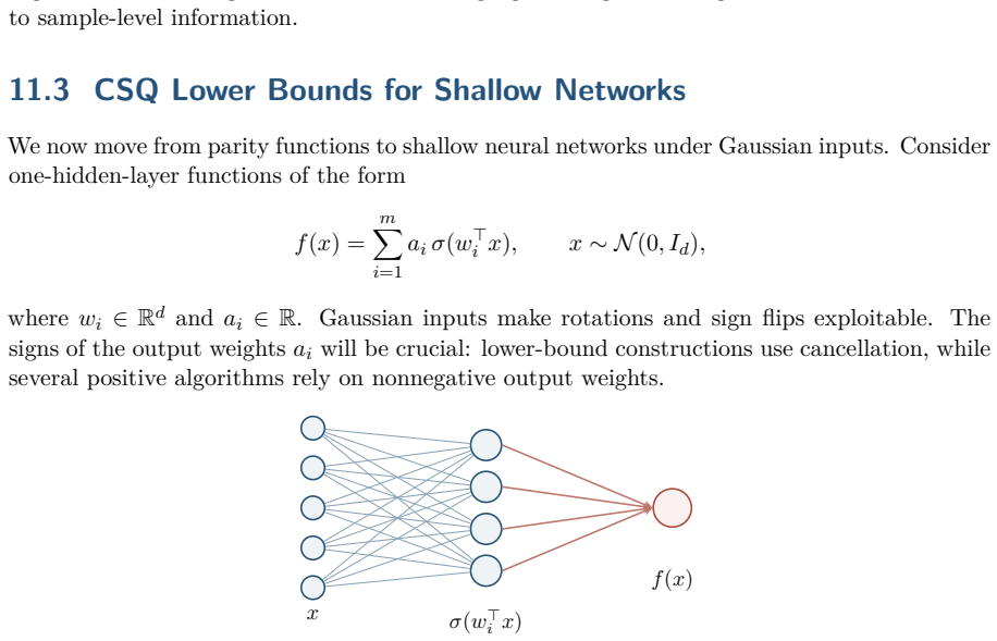
Figure 11.10. Figure 11.10: A one-hidden-layer network under Gaussian inputs. The lower bounds construct many such functions with hidden parity-like sign patterns. Theorem 11.7 (Informal CSQ lower bound under Gaussians). For common activations such as sigmoid or ReLU, any CSQ algorithm learni…
Figure 11.11
Figure 11.11. Figure 11.11: The hidden subset S has size r = dlog2 me. The number of possible subsets is superpolynomial in m when d is large. There are 2 r ≤ 2m hidden units in gS. The output coefficients χ(ω) ∈ {±1} create cancel￾lation, while the Gaussian input distribution supplies sign s…
Figure 11.12
Figure 11.12. Figure 11.12: A sign flip on selected coordinates multiplies gS by the parity of the flip pattern. Lemma 11.11 (Pairwise orthogonality). If S 6= T, then Ex∼N (0,Id) [gS(x)gT (x)] = 0. Proof. Let z be uniformly distributed on {±1} d , independent of x. Since a standard Gaussian i…
Figure 11.13
Figure 11.13. Figure 11.13: The parity-weighted construction acts as a filter, canceling lower interactions and preserving a selected high-degree component. Putting the pieces together, the family {gS : |S| = r} has ℓ = [PITH_FULL_IMAGE:figures/full_fig_p165_11_13.png]
Figure 11.14
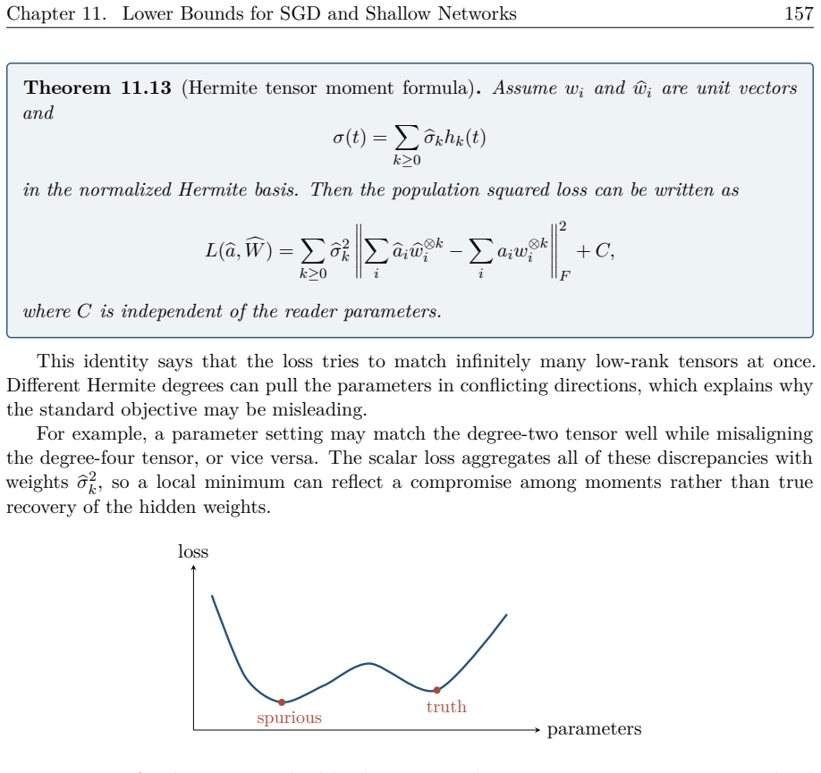
Figure 11.14. Figure 11.14: A schematic standard landscape: matching some moments can create a local minimum that does not recover the teacher parameters. Landscape design changes the objective so that the relevant low-order moment structure has benign critical points. The design principle is…
Figure 11.15
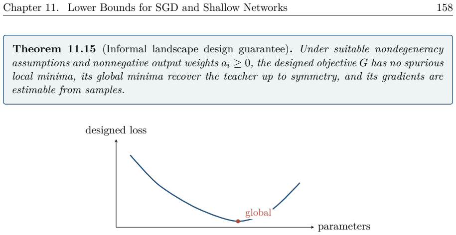
Figure 11.15. Figure 11.15: A schematic designed landscape. Selecting specific Hermite degrees and using nonnegative weights removes the cancellation responsible for the lower-bound construction. This contrast is a major lesson of the chapter. The CSQ lower-bound family uses aω = χ(ω) ∈ {±1},…
Figure 11.16
Figure 11.16. Figure 11.16: Response-weighted covariance vanishes on directions outside the teacher span V . Proposition 11.17 (Positive trace creates a signal direction). Suppose the filter ψ(y) = 1{|y|≥τ} selects examples for which kΠV xk 2 ≥ 2m. Then Mψ has a positive eigenvalue, and every…
Figure 11.17
Figure 11.17. Figure 11.17: Conditioning or filtering on large response breaks spherical symmetry along the teacher subspace, so PCA can find a direction in V . Stein’s lemma explains why second-order response-weighted covariance detects active direc￾tions. Lemma 11.18 (Stein identity). If X …
Figure 12.1
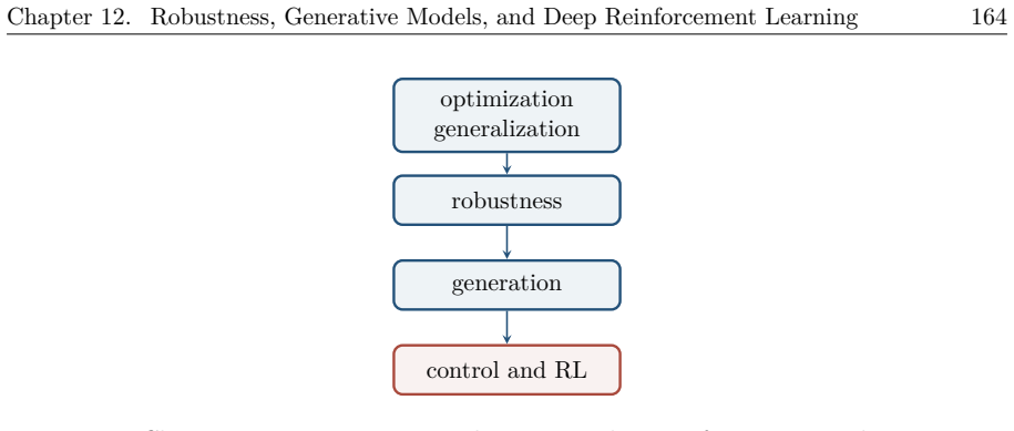
Figure 12.1. Figure 12.1: Chapter 10 is a turning point: the monograph moves from supervised optimization and generalization toward robustness, generation, and control. statistical learning game against nature interactive learning new actors: adversaries, discriminators, and environments [P…
Figure 12.2
Figure 12.2. Figure 12.2: The later topics embed networks inside games and feedback systems, not only inside passive supervised learning problems. In all three cases the objective is no longer just a single empirical average over fixed examples. Geometry, dynamics, and model misspecification…
Figure 12.3
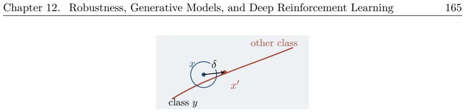
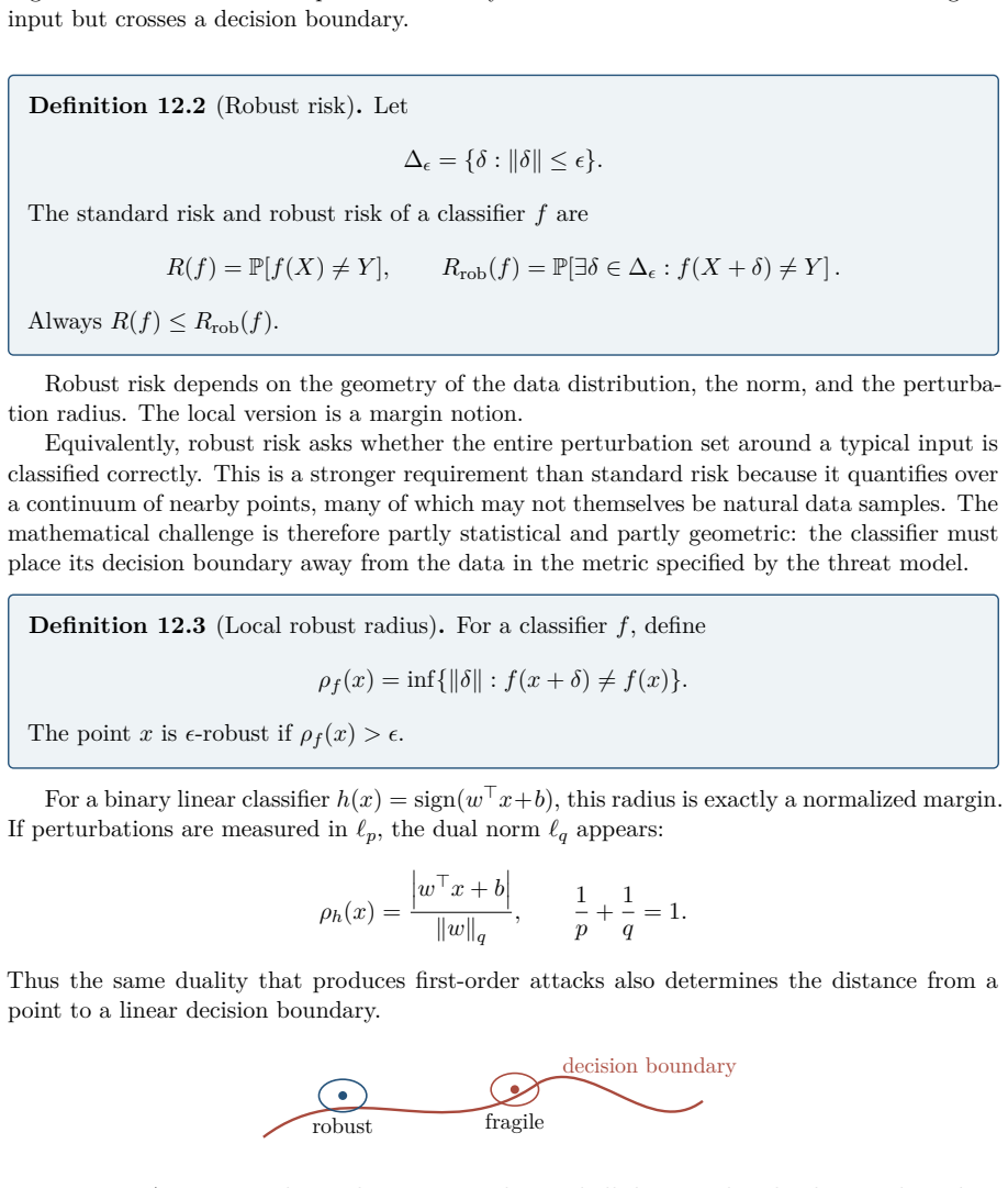
Figure 12.3. Figure 12.3: An adversarial perturbation stays inside a small norm ball around the original input but crosses a decision boundary. Definition 12.2 (Robust risk). Let ∆ϵ = {δ : kδk ≤ ϵ}. The standard risk and robust risk of a classifier f are R(f) = P[f(X) 6= Y ], Rrob(f) = P[∃δ …
Figure 12.4
Figure 12.4. Figure 12.4: A point is robust when its perturbation ball does not hit the decision boundary. Geometrically, robust training tries to move boundaries away from the data manifold. Proposition 12.4 (Dual-norm first-order attack). For differentiable loss ℓ(x, y), the linear [PITH_…
Figure 12.5
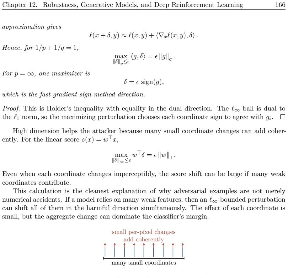
Figure 12.5. Figure 12.5: The ℓ∞ perturbation budget can change many coordinates at once, producing a large aggregate score shift [PITH_FULL_IMAGE:figures/full_fig_p175_12_5.png]
Figure 12.6
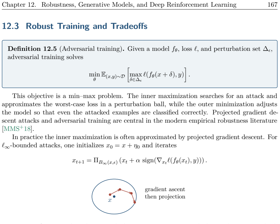
Figure 12.6. Figure 12.6: A projected-gradient attack alternates ascent steps on the loss with projection back into the perturbation ball. Definition 12.6 (Robustness certificate). A certificate proves that, for a given point x, f(x + δ) = f(x) for all kδk ≤ ϵ. It is a rigorous lower bound o…
Figure 12.7
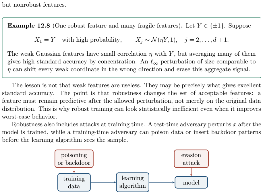
Figure 12.7. Figure 12.7: A schematic robustness–accuracy tradeoff. Robust learning may discard predictive but nonrobust features. Example 12.8 (One robust feature and many fragile features). Let Y ∈ {±1}. Suppose X1 = Y with high probability, Xj ∼ N (ηY, 1), j = 2, . . . , d + 1. The weak G…
Figure 12.8
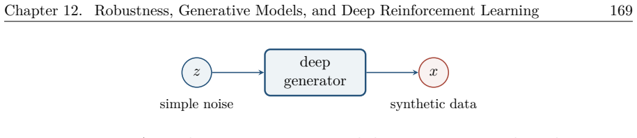
Figure 12.8. Figure 12.8: Robustness includes both test-time evasion attacks and training-time data attacks such as poisoning or backdoors. 12.4 Generative Modeling Generative modeling replaces prediction by distribution learning. Given samples x1, . . . , xn ∼ Pdata, a generator Gθ : R k → …
Figure 12.9
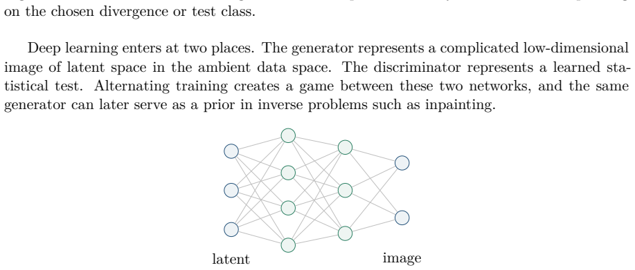
Figure 12.9. Figure 12.9: An implicit generator maps simple latent noise into synthetic data. The phrase “realistic sample” hides a mathematical choice: which distance or divergence between distributions should be optimized? Common choices include DKL(PdatakPθ), DJS(Pdata, Pθ), W1(Pdata, Pθ)…
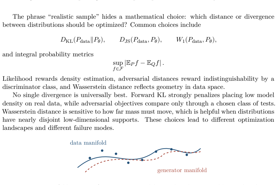
Figure 12.10
Figure 12.10. Figure 12.10: Manifold intuition for generative modeling: a low-dimensional latent distribution is mapped into data space and should align with the true data manifold. Definition 12.9 (Maximum likelihood). For a tractable density pθ(x), maximum likelihood solves max θ 1 n Xn i=1…
Figure 12.11
Figure 12.11. Figure 12.11: Implicit models make sampling easy while leaving likelihood evaluation unavail￾able or expensive. likelihood models latent-variable models adversarial models score and diffusion [PITH_FULL_IMAGE:figures/full_fig_p179_12_11.png]
Figure 12.12
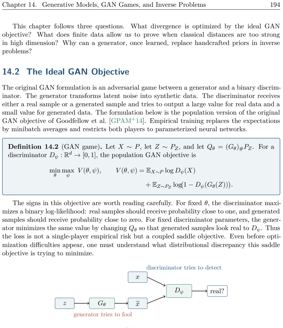
Figure 12.12. Figure 12.12: A taxonomy of generative models. Different approaches make density, sampling, inference, or comparison tractable. 12.5 GAN Theory Definition 12.11 (GAN minimax objective). Generative adversarial networks solve min G max D [Ex∼Pdata log D(x) + Ez∼Pz log(1 − D(G(z)))…
Figure 12.13
Figure 12.13. Figure 12.13: The GAN game pits a generator against a discriminator [PITH_FULL_IMAGE:figures/full_fig_p179_12_13.png]
Figure 12.14
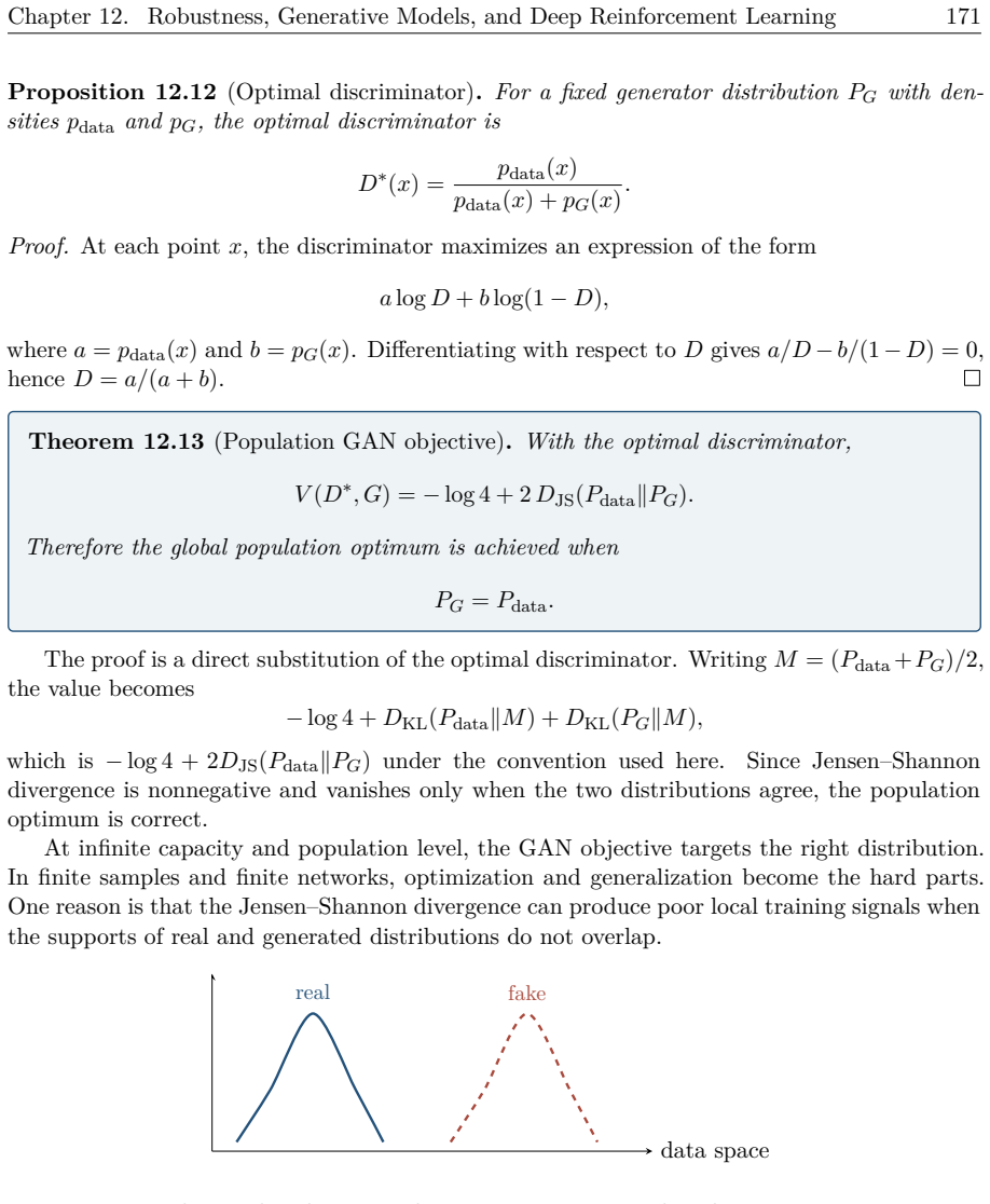
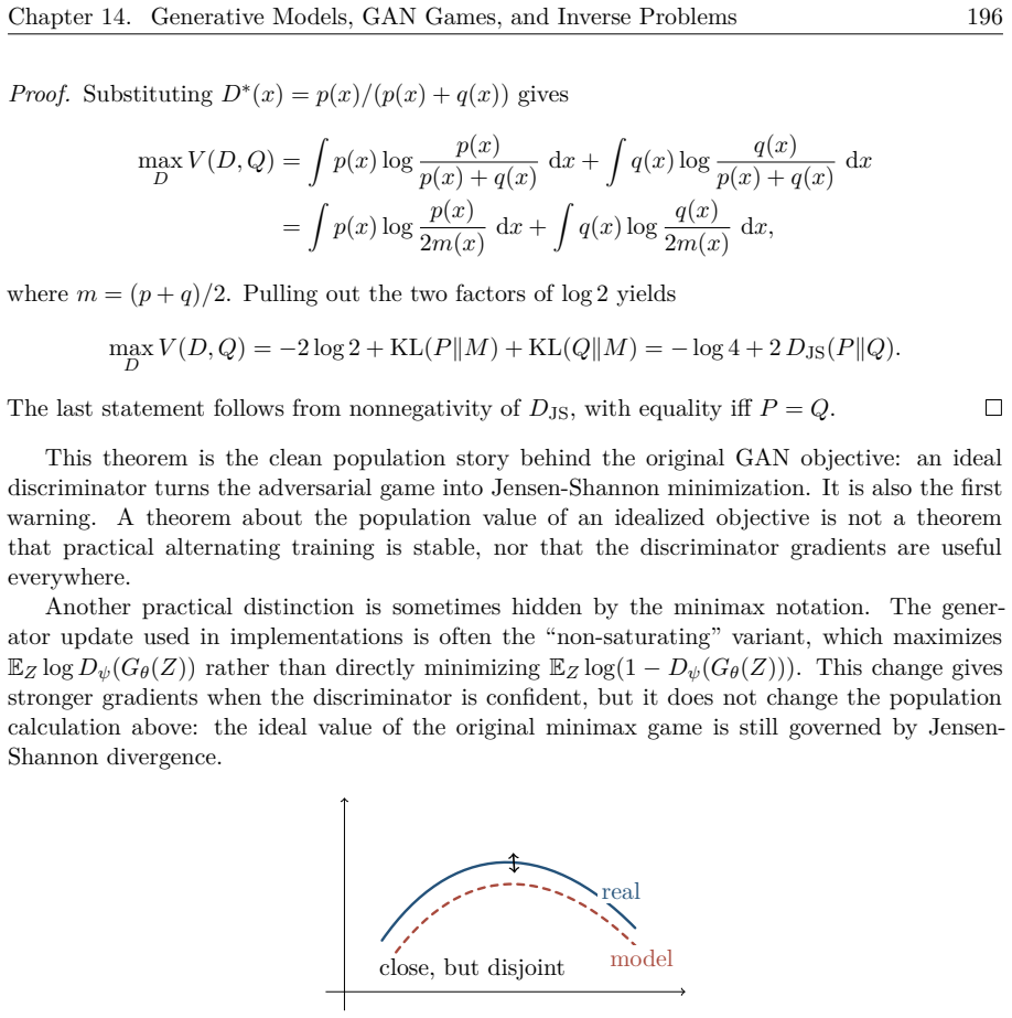
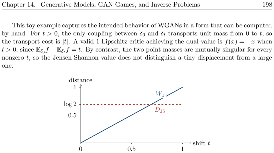
Figure 12.14. Figure 12.14: When real and generated supports are separated, a discriminator can separate them too well and the generator may receive weak or unstable gradients. Definition 12.14 (Earth-mover distance). The 1-Wasserstein distance is W1(P, Q) = inf π∈Π(P,Q) E(X,Y )∼π [PITH_FULL…
Figure 12.15
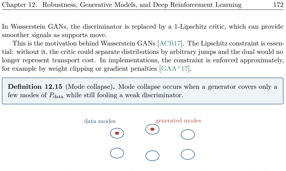
Figure 12.15. Figure 12.15: Mode collapse is a coverage failure: the generated distribution has high fidelity in a few regions but misses other modes. Generalization in GANs is naturally phrased through a discriminator class F, which defines the integral probability metric dF (P, Q) = sup f∈F…
Figure 12.16
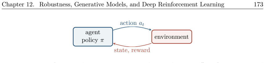
Figure 12.16. Figure 12.16: Reinforcement learning is interactive: the agent’s action affects future states and rewards. Definition 12.17 (Return, value, and Q-value). For a policy π, J(π) = Eπ "X∞ t=0 γ t r(st , at) # . The value and action-value functions are V π (s) = Eπ "X∞ t=0 γ t rt | s…
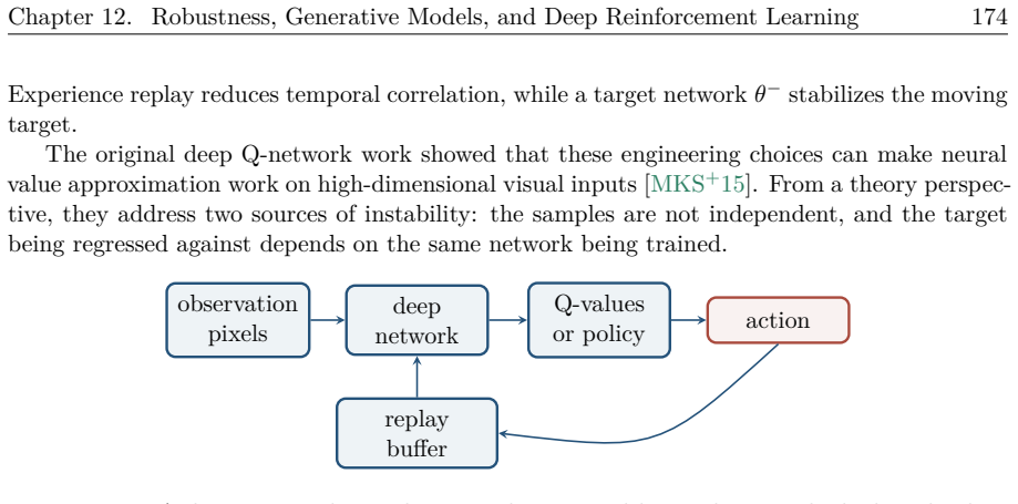
Figure 12.17
Figure 12.17. Figure 12.17: A deep RL pipeline. The network is trained by gradient methods, but the data distribution is generated by the agent’s own policy. Deep RL is difficult both statistically and computationally. Data are dependent, exploration affects what is observed, rewards may be s…
Figure 12.18
Figure 12.18. Figure 12.18: Robustness, GANs, and RL all replace passive supervised learning by a coupled system with feedback. Several open questions remain central. Can robust training avoid losing useful nonrobust features? Which distributional metrics best predict human-perceived sample q…
Figure 13.1
Figure 13.1. Figure 13.1: A small perturbation can move an input across a learned decision boundary. The mathematical issue is not only the size of δ, but the interaction between the metric, the data distribution, and the classifier. training data learner model prediction poisoning evasion …
Figure 13.2
Figure 13.2. Figure 13.2: Two adversarial threat models. Poisoning attacks corrupt the training sample; evasion attacks perturb an input after the model has been trained. Definition 13.1 (Adversarial example). For a classifier f : R d → [K], an input x with true label y, a norm k·k, and a pe…
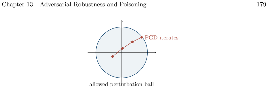
Figure 13.3
Figure 13.3. Figure 13.3: A PGD attack alternates ascent steps on the loss with projection back to the allowed perturbation ball. + + + + − − − − linear robust [PITH_FULL_IMAGE:figures/full_fig_p188_13_3.png]
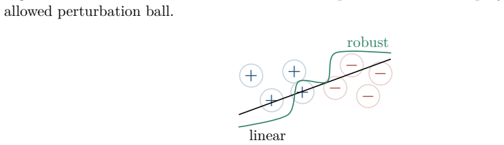
Figure 13.4
Figure 13.4. Figure 13.4: Robust training can require moving the decision boundary away from every per￾turbation ball, which may create a more complex separator. A certification method proves a lower bound rf (x) ≥ r, without relying on the success or failure of a particular attack algorithm…
Figure 13.5
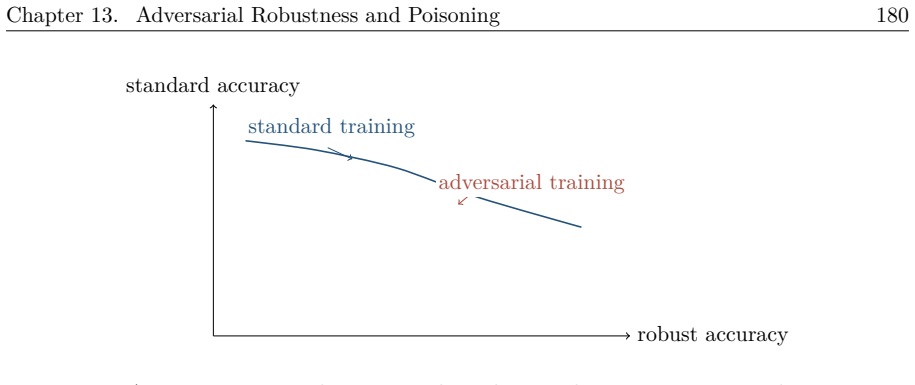
Figure 13.5. Figure 13.5: A common empirical pattern is that adversarial training improves robust accuracy but can reduce clean standard accuracy. u σ(u) ℓ u ReLU convex relaxation [PITH_FULL_IMAGE:figures/full_fig_p189_13_5.png]
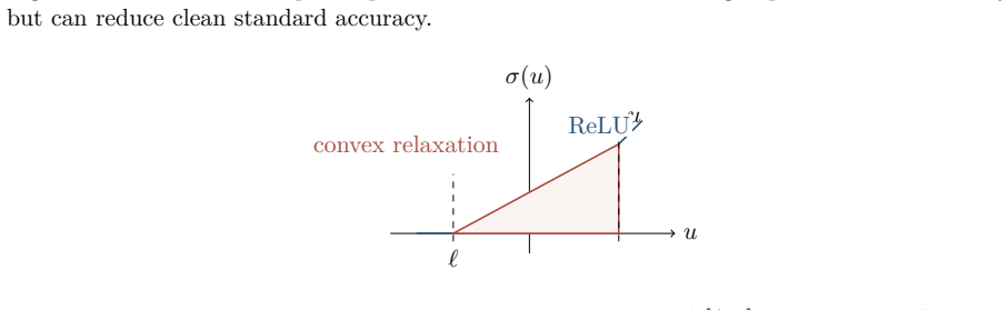
Figure 13.6
Figure 13.6. Figure 13.6: For an ambiguous ReLU with preactivation interval [ℓ, u], the convex hull gives a sound outer relaxation. bounds, linear relaxations, and convex outer polytopes all follow this pattern: {f(x + δ) : kδk ≤ ϵ} ⊆ Prelax. If the relaxed set still has positive margins, th…
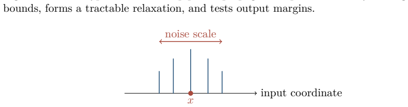
Figure 13.7
Figure 13.7. Figure 13.7: A typical certificate pipeline propagates input uncertainty through activation bounds, forms a tractable relaxation, and tests output margins. input coordinate x noise scale [PITH_FULL_IMAGE:figures/full_fig_p190_13_7.png]
Figure 13.8
Figure 13.8. Figure 13.8: Randomization averages predictions around x. The scale of the noise controls both stability and information loss. Proof. For kx 0 − xk ≤ ϵ, mj (x 0 ) ≥ mj (x) − Lj [PITH_FULL_IMAGE:figures/full_fig_p190_13_8.png]
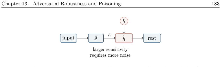
Figure 13.9
Figure 13.9. Figure 13.9: Adding noise to an intermediate layer can make the randomized classifier stable. The required noise scale is controlled by the sensitivity of the preceding map. noise scale certified accuracy best balance too much noise too little radius [PITH_FULL_IMAGE:figures/fu…
Figure 13.10
Figure 13.10. Figure 13.10: Randomized smoothing has a tradeoff: too little noise gives a weak certificate, while too much noise destroys class information. Definition 13.11 (Smoothed classifier). Given a base classifier h and Gaussian noise η ∼ N (0, σ2 I), the smoothed classifier is g(x) = …
Figure 13.11
Figure 13.11. Figure 13.11: Different smoothing distributions certify different perturbation geometries. Gaus￾sian balls are only one case. + + + + + + − − − − − − 1 R label is encoded by radius [PITH_FULL_IMAGE:figures/full_fig_p193_13_11.png]
Figure 13.12
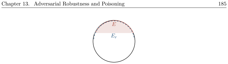
Figure 13.12. Figure 13.12: The adversarial-spheres toy model separates two classes by radius. It isolates geometric effects from image semantics. 13.5 High-Dimensional Limits The chapter next asks whether adversarial examples are an accident of current training methods or a geometric feature…
Figure 13.13
Figure 13.13. Figure 13.13: Reference-note intuition for spherical expansion: spherical caps are the hardest sets to expand, so concentration of measure makes most of the sphere close to a large enough error set. data manifold nearby adversarial set [PITH_FULL_IMAGE:figures/full_fig_p194_13_…
Figure 13.14
Figure 13.14. Figure 13.14: The geometry of real data may be closer to a structured manifold than to a uniform high-dimensional sphere. The theorem should be interpreted as a measure-concentration statement, not as a claim about a particular classifier architecture. It says that once the erro…
Figure 13.15
Figure 13.15. Figure 13.15: Robust learning mixes geometric, optimization, and computational difficulties. 13.6 Poisoning and Robust Statistics The second half of the chapter changes the location of the attack. Instead of perturbing a test input, the adversary corrupts the training sample. In…
Figure 13.16
Figure 13.16. Figure 13.16: A small corrupted bump far from the clean distribution can destroy the mean and variance, while median-based estimates remain stable. Theorem 13.18 (Robust Gaussian estimation). Given ϵ-corrupted samples from a high￾dimensional Gaussian N (µ, Σ), there are polynomi…
Figure 13.17
Figure 13.17. Figure 13.17: Spectral signatures: poisoned examples can create an anomalous low-rank direc￾tion in hidden feature space. detectable low-rank deviation. Remark 13.20 (From robust statistics to deep nets). The statistical filtering step is only as good as the representation on wh…
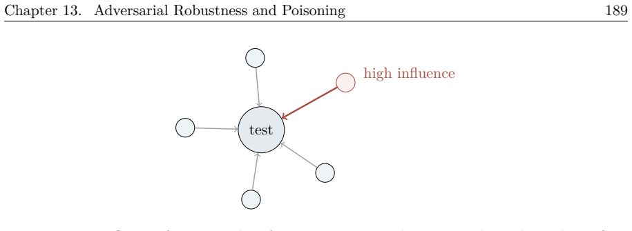
Figure 13.18
Figure 13.18. Figure 13.18: Influence functions identify training points whose upweighting has a large first￾order effect on a test prediction. Threat Mathematical object Typical defense Evasion local input ball adversarial training, certificates Random noise smoothed decision rule probabilit…
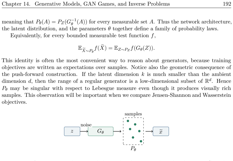
Figure 14.1
Figure 14.1. Figure 14.1: A generator pushes a simple latent distribution PZ through a deep map Gθ, induc￾ing the model law Pθ. This viewpoint is useful because it separates two tasks that are often blurred in practice. First, one must choose a discrepancy that says when two probability laws…
Figure 14.2
Figure 14.2. Figure 14.2: The indistinguishability viewpoint: a test class F defines what differences between real and generated data are visible. Generative adversarial networks (GANs) instantiate this idea by making the tests neural networks. The discriminator or critic is not merely an au…
Figure 14.3
Figure 14.3. Figure 14.3: A distribution-matching lens. The same pair of laws may look close or far depending on the chosen divergence or test class. Deep learning enters at two places. The generator represents a complicated low-dimensional image of latent space in the ambient data space. Th…
Figure 14.4
Figure 14.4. Figure 14.4: A deep generator is a parameterized nonlinear map from latent variables to data. Its range can model a complicated low-dimensional set in R d [PITH_FULL_IMAGE:figures/full_fig_p202_14_4.png]
Figure 14.5
Figure 14.5. Figure 14.5: The adversarial setup in a GAN. The discriminator is trained to distinguish P from Qθ; the generator is trained to make that distinction hard. To understand the population objective, first freeze the generator and optimize over all possible discriminators. This idea…
Figure 14.6
Figure 14.6. Figure 14.6: Two low-dimensional manifolds can be geometrically close and still have disjoint supports. Jensen-Shannon divergence then saturates even though moving one manifold toward the other should be meaningful. The geometric issue is especially visible in high dimension. Da…
Figure 14.7
Figure 14.7. Figure 14.7: Transport intuition for W1. A coupling specifies how to move probability mass from P to Q, and the distance is the minimum expected transport cost. For generative modeling, the most important form of W1 is its dual representation. Theorem 14.8 (Kantorovich-Rubinstei…
Figure 14.8
Figure 14.8. Figure 14.8: For P = δ0 and Qt = δt , Wasserstein distance gives a linear signal in t, while Jensen-Shannon divergence is saturated for every nonzero t. In practice, enforcing the exact Lipschitz constraint is difficult. The original WGAN used weight clipping. Later variants int…
Figure 14.9
Figure 14.9. Figure 14.9: Lipschitz control limits the critic’s slope. Practical WGANs approximate this constraint by clipping, gradient penalties, or spectral normalization. Remark 14.10 (What the Wasserstein objective does and does not solve). Replacing Jensen￾Shannon divergence by W1 addr…
Figure 14.10
Figure 14.10. Figure 14.10: A continuous population and a finite empirical distribution have different sup￾ports. Strong distributional distances may see this support mismatch before they see statistical usefulness. Proposition 14.11 (Strong distances can mislead). Let P = N (0, Id/d), and le…
Figure 14.11
Figure 14.11. Figure 14.11: The covering argument behind neural discriminator generalization. Concentration is proved on a finite net and then extended to the full class by Lipschitzness. The reference notes emphasize the same idea in game-theoretic language. If a generator can approximate po…
Figure 14.12
Figure 14.12. Figure 14.12: A generator mixture can be folded into one larger generator by using part of the latent input as a selector. Equilibrium existence is not the same as training convergence. The toy game min x max y xy [PITH_FULL_IMAGE:figures/full_fig_p211_14_12.png]
Figure 14.13
Figure 14.13. Figure 14.13: In the bilinear game minx maxy xy, gradient descent-ascent rotates around the equilibrium. Game-theoretic existence results therefore do not by themselves guarantee stable GAN training. This distinction matters. The finite-sample and equilibrium results give struct…
Figure 14.14
Figure 14.14. Figure 14.14: Generative compressed sensing searches over latent variables, not over all of R d . The recovered signal is constrained to lie in the generator range [PITH_FULL_IMAGE:figures/full_fig_p213_14_14.png]
Figure 14.15
Figure 14.15. Figure 14.15: Inpainting as a measurement problem. The observed pixels define b = Ax; the generator prior supplies plausible missing pixels through G(zb). Generative priors are powerful but not magical. The true signal may not lie near the generator range. The latent optimizatio…
Figure 15.1
Figure 15.1. Figure 15.1: Transformer theory connects approximation, optimization, and generalization to a new question: when does a fixed network implement an adaptive learning algorithm in its activations? Definition 15.1 (In-context learning). Let Cn = ((xi , yi))n i=1 be a context of exa…
Figure 15.2
Figure 15.2. Figure 15.2: In-context learning turns the prompt into temporary data. The model predicts at x⋆ using information routed from the preceding examples. Transformers are particularly well suited to this view because self-attention compares every token with previous tokens, assigns …
Figure 15.3
Figure 15.3. Figure 15.3: Self-attention supplies content-dependent memory access: a query can read from previous tokens according to learned similarity scores. The guiding question for this chapter is: When does a pretrained transformer implement a learning algorithm inside its for￾ward pas…
Figure 15.4
Figure 15.4. Figure 15.4: Scaled dot-product attention computes query-key scores, normalizes them row￾wise, and uses the resulting attention matrix to average value vectors. Definition 15.2 (Causal mask). For an autoregressive transformer, token t is only allowed to attend to positions 1, . …
Figure 15.5
Figure 15.5. Figure 15.5: The causal mask makes the attention matrix lower triangular: a token may read from the past and present, but not from the future. 15.2.2 Blocks and Heads A transformer block alternates communication across positions with local nonlinear transforma￾tions. In the simp…
Figure 15.6
Figure 15.6. Figure 15.6: A transformer block combines communication through attention with token-wise computation through an MLP, both wrapped by residual connections. Multi-head attention repeats the attention operation several times with different learned projections. Heads are not indepe…
Figure 15.7
Figure 15.7. Figure 15.7: Multi-head attention performs several memory reads in parallel and then recom￾bines the resulting features. 15.3 Expressivity and Attention For a query token i, one attention head computes h + i = X j≤i aijvj , aij = exp(q > i kj/ √ dk) P r≤i exp(q > i kr/ √ dk) . T…
Figure 15.8
Figure 15.8. Figure 15.8: An induction-head style circuit first locates a previous matching pattern and then routes the token that followed it. Mechanistic studies of in-context learning have found induction heads in trained transformer language models. The diagram is schematic, but it captu…
Figure 15.9
Figure 15.9. Figure 15.9: Universal ICL results view a transformer as an approximator of learning rules: the prompt is mapped directly to a prediction. The expressivity landscape has three levels. Attention can route information by content￾based lookup. Transformers can represent many formal…
Figure 15.10
Figure 15.10. Figure 15.10: A linear-attention view of the first gradient step: the context is aggregated into a sufficient statistic and then combined with the query. Proof idea. Store xi in key and value features and store yi in value features. The query token collects a context statistic s…
Figure 15.11
Figure 15.11. Figure 15.11: In the algorithmic view, depth corresponds to computation time: successive layers can implement successive optimization steps. Theorem 15.8 (Preconditioned gradient descent, informal). For linear regression prompts, trained transformer architectures can implement u…
Figure 15.12
Figure 15.12. Figure 15.12: The Bayesian view: the context updates beliefs about the latent task, and the prediction integrates over that posterior. Example 15.9 (Linear-Gaussian tasks). Assume w ∼ N(0, τ 2 I), yi = x > i w + ξi , ξi ∼ N(0, σ2 ). Then the posterior mean prediction is E[y⋆ | C…
Figure 15.13
Figure 15.13. Figure 15.13: Algorithm selection in context. The examples reveal a latent task family, and the model routes the prompt through the corresponding rule. Mixture models clarify both the promise and the limitation. Wider pretraining mixtures can improve task identification; rare ta…
Figure 15.14
Figure 15.14. Figure 15.14: Pretraining mixtures matter. A model can learn narrow selection among familiar families while remaining weak in low-support or out-of-mixture regions. 15.6 Generalization and Limits There are at least three axes of generalization. A transformer can be fluent at tok…
Figure 15.15
Figure 15.15. Figure 15.15: In-context learning generalizes along several axes. The ability to continue text is not identical to the ability to infer a task rule [PITH_FULL_IMAGE:figures/full_fig_p229_15_15.png]
Figure 15.16
Figure 15.16. Figure 15.16: Distribution shift for ICL. A prompt from an unseen task family may not be handled by the algorithm selected during pretraining. Remark 15.10 (Limits of the algorithmic view). From a short prompt alone, many task rules can agree on all observed examples but disagre…
Figure 16.1
Figure 16.1. Figure 16.1: Diffusion models and flow matching replace direct density estimation by learned transport along a path of intermediate distributions. Definition 16.1 (Denoising generator). A diffusion model chooses a forward corruption process that maps x0 ∼ pdata to noisy variable…
Figure 16.2
Figure 16.2. Figure 16.2: The diffusion idea: a known noising process moves data toward a simple prior, and a learned reverse process generates data from noise. Definition 16.2 (Continuous transport and flow matching). Let X0 ∼ pbase be a base sample and X1 ∼ pdata a data sample. Flow matchi…
Figure 16.3
Figure 16.3. Figure 16.3: Flow matching learns the velocity field of a chosen path from the base law to the data law. The chapter has three layers. First, we review the discrete DDPM construction. Second, we pass to continuous-time score SDEs and probability-flow ODEs. Third, we formulate fl…
Figure 16.4
Figure 16.4. Figure 16.4: The DDPM forward process is a prescribed noising chain. At large t, the marginal becomes close to a standard Gaussian [PITH_FULL_IMAGE:figures/full_fig_p235_16_4.png]
Figure 16.5
Figure 16.5. Figure 16.5: The simplified DDPM objective is supervised regression: construct a noisy input and ask the network to predict the noise that was added. 16.2.3 Reverse Sampling Sampling uses learned reverse conditionals pθ(xt−1 | xt) = N (µθ(xt , t), Σt) to transform xT ∼ N (0, I) …
Figure 16.6
Figure 16.6. Figure 16.6: Reverse sampling follows a learned Markov chain from Gaussian noise back toward the data distribution. This explains why diffusion models avoid explicit density estimation. They do not need pdata(x) itself. They need local denoising information at many noise levels.…
Figure 16.7
Figure 16.7. Figure 16.7: A score field is local: it points toward regions of larger log-density at each noise level [PITH_FULL_IMAGE:figures/full_fig_p237_16_7.png]
Figure 16.8
Figure 16.8. Figure 16.8: The reverse SDE and the probability-flow ODE differ pathwise but agree at the level of one-time marginal distributions [PITH_FULL_IMAGE:figures/full_fig_p238_16_8.png]
Figure 16.9
Figure 16.9. Figure 16.9: Sampler design balances quality, number of solver steps, stochasticity, and accu￾mulated error. 16.4 Learning Scores 16.4.1 Denoising Score Matching The basic identity behind diffusion training says that Gaussian denoising recovers the score of the corrupted distrib…
Figure 16.10
Figure 16.10. Figure 16.10: Score learning is vector-field regression: a corrupted sample is fed to the network and a denoising target supplies the local field. Several sources of error must be controlled to turn score learning into a guarantee for gener￾ated samples. The learned score may di…
Figure 16.11
Figure 16.11. Figure 16.11: The generated distribution is affected by score estimation error, solver error, and tail or truncation error. Theorem 16.7 (Informal error decomposition). Assume the target density is regular, the score estimator satisfies Z T 0 Ept ksθ(Xt , t) − st(Xt)k 2 dt ≤ ε 2…
Figure 16.12
Figure 16.12. Figure 16.12: Conditional flow matching constructs paths between base and data samples; the conditional velocity is known by design. The flow matching objective is min θ Et,z,x kvθ(Xt , t) − ut(Xt | z, x)k 2 . The notation ut(Xt | z, x) emphasizes that the target is the velocity…
Figure 16.13
Figure 16.13. Figure 16.13: Conditional flow matching is again supervised vector-field regression, now with velocity labels rather than denoising labels. 16.5.3 Rectification and Couplings The simplest independent coupling between z and x may create curved or crossing marginal trajectories. R…
Figure 16.14
Figure 16.14. Figure 16.14: Rectified flow aims to replace curved trajectories by straighter paths, reducing the numerical burden during sampling [PITH_FULL_IMAGE:figures/full_fig_p243_16_14.png]
Figure 16.15
Figure 16.15. Figure 16.15: Minibatch optimal-transport couplings try to pair base and data samples so that the conditional paths are easier to learn. 16.6 Unification and Solvers 16.6.1 Two Views of the Same Transport Problem Diffusion and flow matching can be placed side by side: diffusion/…
Figure 16.16
Figure 16.16. Figure 16.16: Stochastic interpolants unify deterministic flows and diffusion-like paths by com￾bining interpolation with optional injected noise. 16.6.2 Solver and Neural Error Given a learned field vθ, ODE sampling solves X˙ t = vθ(Xt , t), X0 ∼ pbase. If the true field is Lip…
Figure 16.17
Figure 16.17. Figure 16.17: Classifier-free guidance modifies the local score or velocity direction to trade diversity for condition fidelity. 16.6.4 When Is Flow Matching Easier? A path is easy when its marginal velocity field is smooth, low-curvature, and aligned with the data geometry. Ind…
Figure 16.18
Figure 16.18. Figure 16.18: A concept map for diffusion and flow matching: choose a path, learn a field, solve dynamics, and generate samples. 16.7 Limitations, Connections, and Outlook 16.7.1 What Current Theory Explains Current theory explains several important pieces. Denoising losses iden…
Figure 17.1
Figure 17.1. Figure 17.1: A deployment budget can be spent before deployment, through model size and data, or during deployment, through test-time computation. Definition 17.1 (Training-time and test-time scaling). Training-time scaling chooses N and D under a training compute budget Ctrain …
Figure 17.2
Figure 17.2. Figure 17.2: The workflow of scaling experiments: measure smaller runs, fit laws, allocate resources, and update the frontier [PITH_FULL_IMAGE:figures/full_fig_p250_17_2.png]
Figure 17.3
Figure 17.3. Figure 17.3: On log-log axes, excess loss under a power law is approximately linear. A change of regime changes the slope. For language models, a common separable approximation is L(N, D) = L∞ + AN −α + BD−β . The first term after the floor represents capacity or approximation e…
Figure 17.4
Figure 17.4. Figure 17.4: Scaling-law fitting is a closed loop: small runs estimate the law, larger predictions test it, and the residuals guide new experiments. Remark 17.3 (What power laws do not say). A fitted power law summarizes a regime; it does not identify the mechanism by itself. Da…
Figure 17.5
Figure 17.5. Figure 17.5: Under a fixed training compute budget, increasing model size and increasing data are competing uses of the same resource. Proposition 17.4 (Balanced allocation). Assume L(N, D) − L∞ = AN −α + BD−β , ND = C. Then the compute-optimal allocation obeys N⋆ ∝ C β/(α+β) , …
Figure 17.6
Figure 17.6. Figure 17.6: Compute-optimal training balances marginal returns from model size and data [PITH_FULL_IMAGE:figures/full_fig_p253_17_6.png]
Figure 17.7
Figure 17.7. Figure 17.7: A historical shift: more data per parameter moved the compute-optimal frontier away from undertrained large models. High-quality data may be finite. If D must exceed unique data, training repeats examples. Repetition can still help, but marginal returns often degrad…
Figure 17.8
Figure 17.8. Figure 17.8: Data-constrained scaling distinguishes unique data, repeated tokens, synthetic tokens, and effective data quality [PITH_FULL_IMAGE:figures/full_fig_p254_17_8.png]
Figure 17.9
Figure 17.9. Figure 17.9: A spectral view: learning more modes leaves a smaller tail of unlearned energy, and algebraic tails can produce power-law curves. This picture connects scaling laws to the themes of previous chapters. A useful mental decomposition is L − L∞ ≈ approximation | {z } N …
Figure 17.10
Figure 17.10. Figure 17.10: Effective dimension counts how many eigen-directions are visible at a given scale. Proposition 17.6 (Spectral tail to learning curve). Suppose the remaining target energy after learning m modes satisfies X j>m a 2 j ≤ C0m−r . If the number of reliably learned modes…
Figure 17.11
Figure 17.11. Figure 17.11: Scaling extrapolation is fragile when the experimental regime changes [PITH_FULL_IMAGE:figures/full_fig_p256_17_11.png]
Figure 17.12
Figure 17.12. Figure 17.12: Test-time compute treats inference as a small decision process: generate candi￾dates, check them, and possibly continue. Lemma 17.8 (Oracle pass probability). If each independent sample solves a problem with probability p, then the probability that at least one of …
Figure 17.13
Figure 17.13. Figure 17.13: Repeated sampling has diminishing returns: gains are largest when the base success probability is neither tiny nor already close to one. 17.5.2 Self-Consistency and Verifiers Self-consistency samples multiple reasoning traces and aggregates their final answers by m…
Figure 17.14
Figure 17.14. Figure 17.14: Self-consistency spends compute on diverse traces and aggregates the final an￾swers. Proposition 17.9 (Selection matters). Let Y1, . . . , YK be candidate answers with verifier scores R(Yi). A verifier-guided best-of-K policy outputs bY = arg max 1≤i≤K R(Yi). Impro…
Figure 17.15
Figure 17.15. Figure 17.15: Search over thoughts allocates inference compute to branching, evaluating, and pruning partial solutions. 17.6 Joint Scaling of Training and Inference 17.6.1 An Inference-Aware Objective For a trained model and a test-time policy π, write the deployment loss as Lde…
Figure 17.16
Figure 17.16. Figure 17.16: Deployment quality depends on several axes: model size, data, number of at￾tempts, and depth of deliberation or search. 17.6.2 Thinking Versus Size If extra inference compute raises solution probability more cheaply than increasing model size, a smaller model with …
Figure 17.17
Figure 17.17. Figure 17.17: A smaller but search-friendly system can beat a larger base model when inference compute has higher marginal return. The policy must also know when to stop thinking. An adaptive test-time policy spends a low budget on easy queries and a high budget on hard ones. Ca…
Figure 17.18
Figure 17.18. Figure 17.18: Adaptive inference routes easy queries to cheap answers and hard queries to more expensive deliberation. 17.6.3 Qualitative Regimes The return to test-time compute depends strongly on base skill. If the base model is too weak, sampling mostly repeats failures. At m…
Figure 17.19
Figure 17.19. Figure 17.19: A phase diagram for inference scaling: test-time compute is most valuable when the base model is competent but not saturated. fit empirical laws choose N, D test-time policy deployed frontier measure, allocate, deploy, and update [PITH_FULL_IMAGE:figures/full_fig_…
Figure 17.20
Figure 17.20. Figure 17.20: Joint scaling closes the loop between empirical measurement, training allocation, inference policy, and deployed performance [PITH_FULL_IMAGE:figures/full_fig_p261_17_20.png]
Figure 18.1
Figure 18.1. Figure 18.1: Mechanistic interpretability refines behavioral descriptions into features and causal circuits. The lower level is not automatically better: it must still explain the observed behavior. The chapter follows the route in figure 18.2. We first review circuits and inter…
Figure 18.2
Figure 18.2. Figure 18.2: The chapter moves from observable behavior to hidden states, sparse features, and causal feature graphs. 18.2 Circuits and Interventions 18.2.1 Residual Streams and Features Let x1:T be a token sequence and let rℓ(t) ∈ R d denote the residual stream at layer ℓ and p…
Figure 18.3
Figure 18.3. Figure 18.3: A circuit claim is causal: the name feature, the attention head, and the copy feature are proposed to mediate a target logit. The figure is schematic; real transformer circuits often use many positions and layers. 18.2.2 Activation Patching Activation patching is th…
Figure 18.4
Figure 18.4. Figure 18.4: Activation patching copies an internal state from a clean run into a corrupted run and measures whether the behavior is restored. Patching is most informative when the clean and corrupted inputs differ in a controlled way. For an induction-head experiment, a clean p…
Figure 18.5
Figure 18.5. Figure 18.5: An induction-head motif: one part of the circuit matches the repeated token A, and another part copies the following token B into the current position. Remark 18.5 (What interventions prove). Strong evidence for a circuit comes from a pattern of interventions: patch…
Figure 18.6
Figure 18.6. Figure 18.6: Polysemanticity occurs when one neuron is associated with several apparently different features. Superposition explains how this can happen when a model stores many sparse features in fewer dimensions. The central question is whether n > d useful features can be rep…
Figure 18.7
Figure 18.7. Figure 18.7: Five feature directions can be packed into a two-dimensional hidden space. The price is nonzero inner products, hence interference when multiple features are active together [PITH_FULL_IMAGE:figures/full_fig_p270_18_7.png]
Figure 18.8
Figure 18.8. Figure 18.8: A schematic phase diagram for feature density and dimension pressure. As features become dense or dimensions become scarce, the model is pushed toward superposition. Superposition can be understood as compression. It lets a model store many rare features, use limite…
Figure 18
Figure 18. Figure 18: figure 18.8 [PITH_FULL_IMAGE:figures/full_fig_p271_18.png]
Figure 18.9
Figure 18.9. Figure 18.9: An SAE maps a dense activation to an overcomplete sparse code and then decodes the code back into the original activation space. 18.4.2 Why Sparsity Helps Without sparsity, the decomposition a = Pm j=1 djzj has many equivalent solutions. If a dense code reconstructs…
Figure 18.10
Figure 18.10. Figure 18.10: Choosing λ balances reconstruction against sparsity. The best interpretability usually lies in an intermediate regime, not at either extreme. Several training choices matter in practice: which layer and token positions provide acti￾vations, whether the residual str…
Figure 18.11
Figure 18.11. Figure 18.11: Feature circuits replace dense activation vectors by sparse variables and then study the causal interactions among those variables. For a scalar logit or score y, local linearization gives a first-order attribution formula: ∆y ≈ X j ∂y ∂zj ∆zj . (18.7) A feature j …
Figure 18.12
Figure 18.12. Figure 18.12: A feature attribution graph summarizes local positive and negative influences among active sparse features and a target logit [PITH_FULL_IMAGE:figures/full_fig_p274_18_12.png]
Figure 18.13
Figure 18.13. Figure 18.13: SAE feature-circuit work is iterative: discover features, interpret them, intervene on them, build graphs, and test the explanation on new data. Example 18.9 (A monosemantic feature claim). A feature is plausibly monosemantic when its top activating examples share …
Figure 18.14
Figure 18.14. Figure 18.14: Evaluation should not confuse interpretability with faithfulness. Human-legible features still need causal and transfer tests. Representation metrics include reconstruction error, fraction of variance explained, average active features, feature activation frequency…
Figure 18.15
Figure 18.15. Figure 18.15: Common SAE failure modes form a loop: dataset choices bias the dictionary, human labels over-interpret features, weak validation permits strong claims, and those claims influence the next dataset. The main theoretical questions are still open. First, under what dis…
Figure 19.1
Figure 19.1. Figure 19.1: Grokking separates fitting the training set from discovering a generalizing internal rule. Definition 19.1 (Grokking phenomenology). A training run exhibits grokking when it reaches near-perfect training accuracy at time ttrain, while near-perfect test accuracy appe…
Figure 19.2
Figure 19.2. Figure 19.2: The visible metric may remain flat while the model builds reusable structure. The delayed jump marks when that structure becomes usable by the readout. Grokking is a meeting point of themes from earlier chapters. Optimization dynamics deter￾mine whether the model ke…
Figure 19.3
Figure 19.3. Figure 19.3: Grokking studies the move from interpolation to structured computation, so it naturally touches optimization, regularization, representation geometry, and emergence. algorithmic tasks grokking curves Fourier mechanisms emergent generalization [PITH_FULL_IMAGE:figur…
Figure 19.4
Figure 19.4. Figure 19.4: The chapter first defines the experimental setup, then analyzes the curves, the modular-arithmetic mechanism, and the connection to emergence. 19.2 Setup and Algorithmic Tasks 19.2.1 Supervised Learning View Let (x, y) ∼ D and train a model fθ : X → Y on S = {(xi , …
Figure 19.5
Figure 19.5. Figure 19.5: Modular addition on Z7 can be viewed as moving around a clock. This reveals periodic structure that a lookup table hides. Two predictors can have the same training loss but very different test behavior. A mem￾orizing solution stores observed labels with little reusa…
Figure 19.6
Figure 19.6. Figure 19.6: Memorization and rule learning are both compatible with interpolation, but only the rule generalizes across the whole modular table. Definition 19.3 (Grokking delay). For a threshold 0 < α < 1, define ttrain = inf{t : acctrain(t) ≥ α}, ttest = inf{t : acctest(t) ≥ α…
Figure 19.7
Figure 19.7. Figure 19.7: The delay ratio compares the time to interpolate with the time to generalize. 19.3 Curves and Phase Transitions 19.3.1 Canonical Curves The canonical grokking curve has a rapid training-accuracy rise, a long plateau, and a late test-accuracy jump. Time is often plot…
Figure 19.8
Figure 19.8. Figure 19.8: A typical grokking curve: the training metric saturates early, while the test metric improves only after a long delay. It is tempting to call this a phase transition. That language is useful only when one specifies a measurable statistic that behaves like an order p…
Figure 19.9
Figure 19.9. Figure 19.9: An order parameter translates a qualitative regime change into a measurable curve [PITH_FULL_IMAGE:figures/full_fig_p284_19_9.png]
Figure 19.10
Figure 19.10. Figure 19.10: Hidden progress measures can improve for a long time before test accuracy crosses the threshold. Proposition 19.5 (Thresholded metrics). Suppose a latent score s(C) improves smoothly with compute or scale C, but a benchmark reports A(C) = 1{s(C) ≥ τ}. Then A(C) can…
Figure 19.11
Figure 19.11. Figure 19.11: A thresholded benchmark can turn gradual capability into an abrupt reported score. 19.4 Mechanisms in Modular Arithmetic 19.4.1 Fourier Coordinates on Zp The reason modular addition is analytically attractive is that the cyclic group has a simple Fourier basis. Let…
Figure 19.12
Figure 19.12. Figure 19.12: A compact circuit computes phases for a and b, combines them, and scores the modular sum. 19.4.2 A Mechanistic Story Mechanistic analyses of modular addition find internal variables that become more sinusoidal and more aligned with the correct Fourier modes before …
Figure 19.13
Figure 19.13. Figure 19.13: A mechanistic progress story: embeddings become circular, phase features com￾bine trigonometrically, and logits become readable as modular answers [PITH_FULL_IMAGE:figures/full_fig_p287_19_13.png]
Figure 19.14
Figure 19.14. Figure 19.14: Progress measures can reveal a shift from memorizing features to algorithmic features before the accuracy jump. Proposition 19.8 (Shared harmonic rule). If a model constructs features approximating χk(a) and χk(b) for several k, then a shallow readout can represent…
Figure 19.15
Figure 19.15. Figure 19.15: Interpolation alone does not determine which solution is selected. Grokking depends on the late-time movement among low-training-loss solutions. Proposition 19.9 (Simplicity bias). Suppose two interpolating predictors fmem and frule satisfy Rb S(fmem) = Rb S(frule)…
Figure 19.16
Figure 19.16. Figure 19.16: Grokking can be interpreted as a slow transition from a lazy fit to a feature￾learning solution [PITH_FULL_IMAGE:figures/full_fig_p289_19_16.png]
Figure 19.17
Figure 19.17. Figure 19.17: Grokking separates the presence of statistical signal from the optimization process that extracts it efficiently. 19.6.2 Emergence and Measurement Large-model benchmarks often report emergent abilities: performance appears near chance for small scales and then jump…
Figure 19.18
Figure 19.18. Figure 19.18: Emergent abilities may reflect a new internal mechanism, a thresholded metric, or both. A sharp score alone is not enough to decide. A useful way to summarize experiments is a phase diagram whose axes are regularization strength and data fraction. Delay is most vis…
Figure 19.19
Figure 19.19. Figure 19.19: A schematic phase diagram: grokking is most visible near the boundary between memorization-dominated training and rule-learning training. 19.7 Measurement, Limits, and Open Questions The right measurements include both external and internal quantities. External met…
Figure 20.1
Figure 20.1. Figure 20.1: A common alignment pipeline first builds capability through pretraining, then teaches instruction following, and finally optimizes against preference information. The first mathematical question is therefore: How does a preference label become an objective for chang…
Figure 20.2
Figure 20.2. Figure 20.2: Preference supervision compares candidate behaviors rather than declaring one response to be the unique target [PITH_FULL_IMAGE:figures/full_fig_p295_20_2.png]
Figure 20.3
Figure 20.3. Figure 20.3: The argument: model preference labels, connect reward optimization to KL control, derive DPO, and then examine the broader method family and its limitations. 20.2 Preference Data and Reward Models Definition 20.2 (Preference dataset). A pairwise preference dataset i…
Figure 20.4
Figure 20.4. Figure 20.4: Reward-model training fits a scalar proxy so that preferred responses receive larger scores than rejected responses. Proposition 20.5 (Preference likelihood is invariant to prompt shifts). For any function c : X → R, the rewards r(x, y) and r 0 (x, y) = r(x, y) + c(…
Figure 20.5
Figure 20.5. Figure 20.5: Preference modeling is statistical estimation under noisy and incomplete feedback. The optimized policy can also change the distribution of future comparisons. 20.3 RLHF as KL-Regularized Control In classical RLHF for language models, the reward model is used as an …
Figure 20.6
Figure 20.6. Figure 20.6: RLHF learns a reward model from preferences and then performs KL-regularized policy optimization. For a prompt x, let πref(· | x) be the reference policy and let r(x, y) be a learned reward [PITH_FULL_IMAGE:figures/full_fig_p298_20_6.png]
Figure 20.7
Figure 20.7. Figure 20.7: A geometric view of RLHF: the policy moves in a reward-improving direction while being penalized for leaving the neighborhood of the reference policy. In large language models the exact maximizer is not computed by enumerating responses. Practical RLHF often uses a …
Figure 20.8
Figure 20.8. Figure 20.8: RLHF explicitly learns a reward and optimizes it by RL; DPO folds the KL-control solution into the preference likelihood. Proposition 20.9 (Reference-corrected log odds). DPO increases the policy log-odds of the preferred response relative to the reference policy. I…
Figure 20.9
Figure 20.9. Figure 20.9: DPO behaves like a contrastive supervised objective, with update size controlled by the current reference-corrected margin. To see this analytically, write the loss on one example as ℓθ = − log σ(βmθ). Then ∇θℓθ = −β [PITH_FULL_IMAGE:figures/full_fig_p302_20_9.png]
Figure 20.10
Figure 20.10. Figure 20.10: The inverse-temperature β converts log-ratio margins into preference logits. Larger values make the logistic transition sharper [PITH_FULL_IMAGE:figures/full_fig_p302_20_10.png]
Figure 20.11
Figure 20.11. Figure 20.11: Direct preference objectives differ in their data format and in how they score policy deviations from a reference. IPO and margins. The logistic DPO loss can continue increasing preference margins when labels are nearly separable. IPO-style views introduce a finite…
Figure 20.12
Figure 20.12. Figure 20.12: Preference objectives balance three pressures: fit the feedback, remain close to the reference behavior, and optimize strongly enough to matter. This family perspective is useful when comparing algorithms. The question is not whether one loss is universally correct…
Figure 20.13
Figure 20.13. Figure 20.13: Reward hacking can be viewed as distribution shift: optimization queries the proxy reward in regions not well constrained by preference data. Reward hacking. Reward hacking occurs when a policy finds responses that score highly under the proxy reward while failing …
Figure 20.14
Figure 20.14. Figure 20.14: Goodhart’s law in schematic form: as the proxy becomes the target, true quality may eventually stop improving or decline. Goodhart’s law is not a theorem about every reward model, but it is a useful warning. If a proxy is selected because it correlates with quality…
Figure 20.15
Figure 20.15. Figure 20.15: Preference optimization is safer when the comparison data cover the responses likely to be produced after optimization. Preference ambiguity. Human preferences are not a single deterministic function. They differ across annotators, cultures, expertise levels, and a…
Figure 20.16
Figure 20.16. Figure 20.16: Preference fit is one ingredient of deployment alignment, but it must be combined with robustness, truthfulness, calibration, and other safety requirements. Remark 20.13 (A practical checklist). During training, monitor KL to the reference, chosen and rejected log-…
Figure 21.1
Figure 21.1. Figure 21.1: OOD generalization asks whether a model trained on observed domains can be trusted on a new deployment domain. The distribution shift creates an extra term beyond ordinary finite-sample generalization. If P is the training distribution and Q is the deployment distri…
Figure 21.2
Figure 21.2. Figure 21.2: Perfect behavior on the training support need not constrain the model’s behavior on deployment support. There are several common names for recurring shift patterns. Under covariate shift, P(X) 6= Q(X) but P(Y | X) is stable. Under label shift, P(Y ) 6= Q(Y ) but P(X…
Figure 21.3
Figure 21.3. Figure 21.3: OOD deployment combines questions from generalization, robustness, representa￾tion learning, in-context adaptation, and alignment. OOD risk adaptation bounds robust learning detect and calibrate foundation models [PITH_FULL_IMAGE:figures/full_fig_p311_21_3.png]
Figure 21.4
Figure 21.4. Figure 21.4: The chapter moves from formal risk to adaptation bounds, robust training, uncer￾tainty, and foundation-model evaluation. 21.2 Environments, Risks, and Shift Models Definition 21.1 (Environment model and OOD risk). Let e ∈ E index a distribution Pe on X × Y. For a pr…
Figure 21.5
Figure 21.5. Figure 21.5: A shortcut feature can be predictive in training environments while being unstable across environments. The example exposes the necessary ingredients for OOD learning. The target should not require unconstrained prediction on a region with no source information; som…
Figure 21.6
Figure 21.6. Figure 21.6: The domain adaptation bound decomposes target error into source error, domain discrepancy, and shared-solution error. The operational interpretation of the discrepancy term leads to domain-adversarial learning. If a domain classifier can easily distinguish source fr…
Figure 21.7
Figure 21.7. Figure 21.7: Domain-adversarial representation learning uses a task head and a domain head to encourage discriminative but domain-invariant features. The adaptation bound also points to an impossibility: making marginals look similar cannot create labels where there is no source…
Figure 21.8
Figure 21.8. Figure 21.8: Group DRO focuses optimization pressure on the high-loss group rather than allowing average performance to hide a subgroup failure. Definition 21.10 (Invariant Risk Minimization). The ideal IRM objective seeks a repre￾sentation Φ such that the same classifier w is o…
Figure 21.9
Figure 21.9. Figure 21.9: A feature whose relation to the label survives environment changes is a better OOD candidate than a shortcut feature. In practice, the exact IRM constraint is difficult to enforce. A common surrogate fixes a scalar classifier and penalizes environment-wise optimalit…
Figure 21.10
Figure 21.10. Figure 21.10: Energy-based detection separates ID and OOD examples by thresholding a scalar score. Predictive uncertainty also changes under dataset shift. A Bayesian or ensemble predictor estimates p(y | x, D) = Z p(y | x, θ) p(θ | D) dθ. Moving away from the training support c…
Figure 21.11
Figure 21.11. Figure 21.11: In-context learning can be viewed as target adaptation using prompt examples and the pretrained prior. For language models, OOD shift is not only a change in input distribution. It can involve new dialects, APIs, laws, tools, adversarial prompt styles, long-context…
Figure 21.12
Figure 21.12. Figure 21.12: OOD robustness for foundation models is an ongoing evaluation and monitoring loop rather than a one-time benchmark score. Recent theory and empirical work asks several related questions. Can a learner test whether a target distribution is safe before trusting a hyp…
Figure 22.1
Figure 22.1. Figure 22.1: Observed emergence can arise from metric thresholding, finite-size critical behavior, or genuine mechanism formation. This chapter takes a deliberately decompositional view. We do not treat “emergence” as an explanation. We treat it as a hypothesis to be broken into…
Figure 22.2
Figure 22.2. Figure 22.2: The chapter’s structure: define the observable, rule out artifacts, study solvable models, analyze training transitions, and formulate research programs. 22.2 Metrics, Slices, and Apparent Jumps The first diagnostic for any emergence claim is the metric. Many benchm…
Figure 22.3
Figure 22.3. Figure 22.3: A discontinuous or thresholded metric can create an apparent jump from a smooth latent score. The diagnostic lesson is simple: before claiming emergence, replace exact-match accuracy by a continuous score when possible, condition on task difficulty, vary the prompt …
Figure 22.4
Figure 22.4. Figure 22.4: Aggregating easy and hard slices can hide smoother slice behavior and create an apparent emergence threshold. In-context learning is another confounder. Some abilities attributed to large-model emer￾gence can be decomposed into memory, linguistic knowledge, and task…
Figure 22.5
Figure 22.5. Figure 22.5: Discrete skill quanta can make one ability appear suddenly while the aggregate loss remains smooth. The multitask sparse parity model makes this idea more concrete. Tasks are basis functions ϕj , and the target is sampled from a heavy-tailed task distribution: f(x) …
Figure 22.6
Figure 22.6. Figure 22.6: A percolation model interprets capability emergence as the appearance of a task￾relevant connected component of learned regularities. For in-context learning, high-dimensional linear attention gives a cleaner limit theory. In linear-regression prompts, take a joint …
Figure 22.7
Figure 22.7. Figure 22.7: Grokking: training accuracy rises early, while test accuracy rises only after a delayed hidden mechanism becomes usable. Definition 22.9 (Lazy-to-rich transition). During early training, a network may behave [PITH_FULL_IMAGE:figures/full_fig_p327_22_7.png]
Figure 22.8
Figure 22.8. Figure 22.8: A two-minima schematic: as training changes the effective landscape, the dominant state can switch discontinuously. Mechanistic interpretability provides a more constructive route. Rather than asking whether a curve jumps, search for continuous progress variables P1…
Figure 22.9
Figure 22.9. Figure 22.9: An induction head matches a previous token and copies the following token, giving an elementary mechanism for in-context pattern continuation. For Markov-chain data, transformers can learn to estimate transition probabilities from context: pb(xt+1 = j | xt = i) ≈ #(…
Figure 22.10
Figure 22.10. Figure 22.10: A schematic phase diagram for in-context learning: task diversity, context length, and architecture determine whether memorization or in-context generalization dominates. Several interpretations of in-context learning coexist. In one view, attention implements grad…
Figure 22.11
Figure 22.11. Figure 22.11: A reference map for emergence theory: empirical claims should be filtered through diagnostics, solvable models, training dynamics, and mechanistic evidence. The open problems are clear. Can we prove finite-size scaling exponents for attention-based models beyond li…

Discussion (0). Continue with ORCID to comment.

Pith tools

Reviewed August 2, 2026 · model on record in the stance chip above.