REVIEW 3 major objections 5 minor 6 references
Exact inference under the perfect phylogeny model
T0 review · 3 major / 5 minor · reviewed 2026-08-14 · deepseek-v4-flash
Pith's one-line read Exact inference under the perfect phylogeny model is achievable by exhaustive enumeration of all small trees.
desk verdict First exact exhaustive inference under the noisy PPM for small trees; the O(q^2) guarantee is real but leans on unproved general-D lemmas, so the paper deserves a serious referee with a request for those proofs. read the letter →
The pith
A machine-rendered reading of the paper's core claim, the machinery that carries it, and where it could break.
The reading
What carries the argument
The engine is a dual active-set path-following algorithm. Using the dual of the projection problem, the cost of a tree is written as $\min_t [t + L(t)]$, where $L(t)$ is the minimum of $\frac12 \sum_i D_{ii}^{-2}(Z_i - Z_{\bar i})^2$ over $Z$ with $Z_i \le t - N_i$; here $\bar i$ is the parent of node $i$ and $N_i$ is the weighted sum of observed frequencies over ancestors of $i$, including $i$. The algorithm starts at a large $t$ with no active constraints and walks downward through critical values $t_1>t_2>\cdots>t_k$ at which a constraint becomes tight. The key structural facts are that $Z^*(t)$ is piecewise linear, each component changes at rate at most $1$, and the active set $B(t)$ grows monotonically and changes at most $q$ times, so extrapolating between critical values and recomputing rates yields the exact minimum in $O(q^2)$ steps. Rates are obtained by decomposing the tree into subtrees separated by active nodes and solving small convex quadratics recursively, while the outer exhaustive search maps integer indices to trees via Prüfer sequences.
What would settle it
Instrument Algorithm 1: for many random trees with random strictly positive diagonal D and random observations, count active-set changes and record all computed rates; if any run exceeds q changes or any rate falls outside [0,1], Theorem 3.4 is false. As a second check, compare Algorithm 1's output for q up to 8 against a direct convex quadratic solver on the same problem (9).
Extended reading notes
Core claim
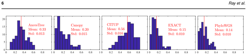
The central claim is Theorem 3.4: Algorithm 1 solves the per-tree cost problem (9) in $O(q^2)$ steps and $O(q)$ memory. Problem (9) is the projection of the noisy observed frequencies $\hat F_O$ onto the set of frequency vectors compatible with a given tree, i.e. minimizing $\|D(\hat F_O - F_O)\|^2$ subject to $F_O = U_{O,O}\tilde M_O$, $\tilde M_O \ge 0$, and a sum constraint; $D$ encodes noise precisions. Computing this projection exactly and fast is what removes the need for heuristics: EXACT enumerates every labeled rooted tree (or every spanning tree of a user-supplied DAG), computes each tree's cost with Algorithm 1, and keeps the top $k$. The paper reports that on the 90 synthetic and 36 real benchmark files, the exact best tree is comparable to the best approximate tool on ancestral-relation error, and that the exact top-$k$ list contains a tree closer to ground truth than the single tree returned by approximate methods.
Load-bearing premise
The O($q^{2}$) bound assumes the unproved lemmas that the optimal dual variables are piecewise linear with slopes in [0,1] and that the active set can change at most q times when the noise weights D are arbitrary positive diagonal; the paper states these proofs are almost identical to those in earlier work but does not include them.
Editorial extensions
If this is right
- For problems with up to about ten mutation clusters, users can obtain the exact maximum-likelihood tree and exact top-$k$ rankings, not just a heuristic best guess.
- The exact ranking of all trees makes it possible to decide whether a discrepancy between model and data is due to the PPM assumptions or to inference error.
- EXACT can serve as a ground-truth benchmark for approximate and sampling-based tools on small PPM instances.
- Because each tree cost is computed to machine precision in a finite number of steps, downstream statistics such as marginal ancestral-relation probabilities inherit exactness up to floating-point arithmetic.
- The same fast per-tree solver can be embedded in an ADMM loop to handle more general convex objectives, as the paper sketches.
Reading between the lines
- If the $O(q^2)$ claim holds for all positive diagonal $D$, a natural extension the paper does not take is exact model averaging over clusterings: instead of fixing one k-means clustering, one could enumerate plausible clusterings and sum exact tree scores, directly testing whether the remaining error gap is caused by clustering.
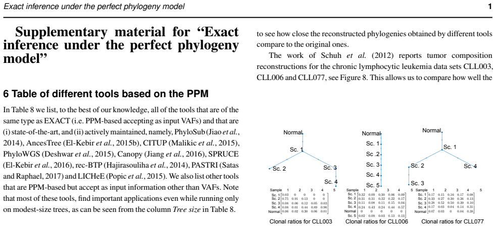
- The exact top-$k$ output suggests a fast exact substitute for MCMC summaries on small instances: posterior probabilities of subclonal presence or ancestral relations can be read off the ranked list, as the paper's CLL example begins to do.
- A stress test that follows naturally is to compare exact tree scores from Algorithm 1 with double-precision iterative solvers on ill-conditioned noise-weight matrices $D$, to locate where finite floating-point arithmetic starts to matter.
Signed reviews
Editorial analysis
A structured set of objections, weighed in public.
Referee Report
Summary. The paper presents EXACT, a GPU-accelerated tool that performs exact inference under the noisy perfect phylogeny model (PPM) on VAF data. The main algorithmic contribution is a fast, non-iterative procedure (Algorithm 1) that computes the exact likelihood cost C(U; F_hat) for a given tree in O(q^2) steps and O(q) memory (Theorem 3.4), using a dual formulation (Theorem 3.3) and a piecewise-linear active-set analysis. EXACT then enumerates all rooted labeled trees of q nodes (via Prüfer sequences) or all spanning trees of a user-supplied DAG, and returns the top-k trees by cost, with BIC-based cluster-number selection. The authors benchmark EXACT against AncesTree, Canopy, CITUP, and PhyloWGS on 90 synthetic and 36 real data sets, reporting competitive or better accuracy and the unique ability to provide exact top-k statistics.
Significance. If the algorithmic claims are fully substantiated, this is a genuinely useful contribution: it is the first tool, to my knowledge, that can exactly evaluate the likelihood of every tree in the q^(q-2) space for biologically relevant small sizes (q up to 10), enabling exact maximum-likelihood tree selection and exact top-k statistics under a noisy PPM. The paper is honest about the scope (small trees, simple k-means clustering) and about the fact that the real data violate the model assumptions. The machine-checkable parts, such as the dual derivation in Theorem 3.3 and the C/CUDA implementation with reproducible benchmark protocol, are strengths. The main significance is conditional on the completeness of the proof of Theorem 3.4, which currently rests on omitted or only sketched lemmas in the supplementary material.
major comments (3)
- [Supp. Mat. Sec. 10 (Lemmas 10.1–10.6)] The correctness of Algorithm 1 and the O(q^2) bound in Theorem 3.4 depend critically on Lemmas 10.1–10.6, especially Lemma 10.5 (monotonicity of the active set B(t), at most q changes) and Lemma 10.6 (fewer than q+1 linear segments). These lemmas are asserted for general strictly positive diagonal D, but no proofs are supplied; the text states that the proofs are 'almost identical' to Lemmas 3.2–3.9 of Jia et al. (2018), and lists only two equation changes. Lemma 10.5 is a combinatorial/monotonicity statement, not an equation change, and the paper does not explain how the D=I proof transfers to general D. Because Theorem 3.4 inherits all of its exactness and complexity guarantees from these lemmas, the central claim is not currently supported by a complete proof. I request that the authors provide the full proofs, or a detailed lemma-by-lemma mapping showing which parts of the Jia et al. proofs are unchanged and which require modification for general diagonal D.
- [Supp. Mat. Sec. 11–12 (Lemma 11.2 and its proof sketch)] Lemma 11.2 is the load-bearing bound that rates c1 of free variables satisfy 0 <= c1 <= 1. This is exactly the property that makes the active set B(t) monotone: if a free variable had rate greater than 1, a node could hit the boundary, leave it, and hit again, potentially creating more than q breakpoints and destroying the O(q^2) claim. The proof given in Supp. Mat. Sec. 12 is only a sketch: the inequality in (39) is asserted, and the 'recursively applying the above inequality' step that produces (40) is not carried out. In particular, it is not shown that the constant C0 in (40) is independent of t, which is necessary for the conclusion c1 <= 1. This is not a merely cosmetic gap; the entire exactness guarantee of Algorithm 1 depends on it. A complete, self-contained proof of Lemma 11.2 for general D is needed.
- [Supp. Mat. Sec. 10 (transfer argument for Theorem 3.4)] The proof of Theorem 3.4 is not included in the manuscript; the text says it is 'exactly the same as a combination of the proofs of Theorems 3.10 and 3.11 in Jia et al. (2018)' with certain substitutions. Given that the two listed equation changes in Supp. Mat. Sec. 10 do not address the structure of Lemmas 10.3, 10.5, and 10.6, the reader cannot verify that the D=I proof transfers to the D != I setting. At minimum, the authors should state precisely which intermediate results from Jia et al. are used in each step of the proof of Theorem 3.4, and supply the missing arguments for the general diagonal D case.
minor comments (5)
- [Supp. Mat. Sec. 12] There is a typo in the proof of Theorem 3.3: 'Moureau's decomposition' should be 'Moreau's decomposition'.
- [Section 3.3, Algorithm 1] The main text says that using L0(t) we find t* such that '1+L0(t*)=0', but Algorithm 1 line 12 computes t* = t_i - (1+L0(t_i))/L00(t_i). This is consistent, but the sentence just before could be clarified to avoid the impression of a sign error.
- [Figures 2–5] Several figures (especially Figures 2, 4, and 5) are low-resolution and axis labels are hard to read; the paper would benefit from larger panels and higher-resolution rendering.
- [Table 5] The runtimes for k=46 are sometimes slightly smaller than for k=1 (e.g., 1.0 vs 1.1 for size 7); this is likely measurement noise, but it would be good to report that runtimes are measured once or to give a variance estimate.
- [Supp. Mat. Sec. 9] The extension to the '≤' constraint in (10) is described briefly; the sentence 'the first required adjustment to the proof of Lemma 3.3' suggests this refers to Theorem 3.3, not Lemma 3.3, and the numbering should be fixed.
Circularity Check
No circular reduction found: the tree likelihood and ranking are derived from the stated noisy-PPM Gaussian model, and the benchmarks are external to the fitted quantities. The only notable issue is proof-deferral to the authors' prior paper for general-D lemmas, which is a completeness gap, not a circularity.
full rationale
The paper derives its per-tree cost C(U;F_hat) from the measurement model in Eqs. (2)-(5) and the constraint F=UM, via Theorems 3.2 and 3.3; it does not define the cost in terms of the ground-truth trees used in the benchmarks. The values D=1/0.06, I(x)=x, Q=0, and the BIC criterion (14) are stated as chosen, not fitted to the labels, and the paper explicitly checks robustness when the BIC penalty is removed. No 'prediction' is a renamed fitted parameter. The one passage that could look circular is Supp. Mat. Sec. 10, where Lemmas 10.1-10.6 are stated and their proofs are omitted because they are 'almost identical' to lemmas in Jia et al. (2018), and where the proof of Theorem 3.4 is said to be 'exactly the same as a combination of the proofs of Theorems 3.10 and 3.11 in Jia et al. (2018)'. This is a self-citation, but it is a proof-deferral rather than a definitional reduction: Jia et al. (2018) is an independent published derivation for D=I, and the two stated equation changes are identifiable for checking. The missing general-D proof is a correctness and completeness risk, not a circular step. Accordingly, no circularity step is scored; the low nonzero score reflects only the minor self-citation in the proof infrastructure.
Assumptions & free parameters
free parameters (2)
- D (precision scaling in Eq. (7)) =
1/0.06 (all entries)
- BIC penalty in Eq. (14) =
p(q-1) log q* (unit weight)
assumptions (6)
- domain assumption Perfect phylogeny: each genome position mutates at most once, so F = U M (Eq. 1)
- domain assumption Observation noise is independent, zero-mean Gaussian with known variance (Eq. 4)
- domain assumption Uniform prior on mutant distributions M (Eq. 5)
- standard math Convex analysis tools: Moreau decomposition and Fenchel dual (Proof of Theorem 3.3)
- ad hoc to paper Lemmas 10.1-10.6 extend from D=I in Jia et al. (2018) to general diagonal D
- standard math Number of rooted labeled trees on q nodes is q^(q-2) (Cayley's formula)
Cite this review
Pith. "Pith review of Exact inference under the perfect phylogeny model." pith.science (2026). https://pith.science/paper/3H3EJMWB
@misc{pith2026190808623,
  author       = {Pith},
  title        = {Pith review of: Exact inference under the perfect phylogeny model},
  year         = {2026},
  howpublished = {\url{https://pith.science/paper/3H3EJMWB}},
  note         = {Machine review of arXiv:1908.08623}
}
read the original abstract
Motivation: Many inference tools use the Perfect Phylogeny Model (PPM) to learn trees from noisy variant allele frequency (VAF) data. Learning in this setting is hard, and existing tools use approximate or heuristic algorithms. An algorithmic improvement is important to help disentangle the limitations of the PPM's assumptions from the limitations in our capacity to learn under it. Results: We make such improvement in the scenario, where the mutations that are relevant for evolution can be clustered into a small number of groups, and the trees to be reconstructed have a small number of nodes. We use a careful combination of algorithms, software, and hardware, to develop EXACT: a tool that can explore the space of all possible phylogenetic trees, and performs exact inference under the PPM with noisy data. EXACT allows users to obtain not just the most-likely tree for some input data, but exact statistics about the distribution of trees that might explain the data. We show that EXACT outperforms several existing tools for this same task. Availability: https://github.com/surjray-repos/EXACT
Figures


Figures from the paper (4 more)



Reference graph
Works this paper leans on
-
[1]
Bento, J., Derbinsky, N., Alonso-Mora, J., and Y edidia, J. S. (2013). A message- passing algorithm for multi-agent trajectory planning. In Advances in neural information processing systems, pages 521–529
work page 2013
-
[2]
Bento, J., Derbinsky, N., Mathy, C., and Y edidia, J. S. (2015). Proximal operators for multi-agent path planning. InAAAI, pages 3657–3663
work page 2015
-
[3]
Boyd, S., Parikh, N., Chu, E., Peleato, B., Eckstein, J., et al.(2011). Distributed optimization and statistical learning via the alternating direction method of multipliers.F oundations and Trends® in Machine Learning,3(1), 1–122. França, G. and Bento, J. (2016). An explicit rate bound for over-relaxed admm. InInformation Theory (ISIT), 2016 IEEE Interna...
work page 2011
-
[4]
Hao, N., Oghbaee, A., Rostami, M., Derbinsky, N., and Bento, J. (2016). Testing fine-grained parallelism for the admm on a factor-graph. InParallel and Distributed Processing Symposium Workshops, 2016 IEEE International, pages 835–844. IEEE
work page 2016
-
[5]
J., Gonda, F., Schmidt, D., Derbinsky, N., Alemi, A
Mathy, C. J., Gonda, F., Schmidt, D., Derbinsky, N., Alemi, A. A., Bento, J., Delle Fave, F. M., and Y edidia, J. S. (2015). Sparta: Fast global planning of collision-avoiding robot trajectories
work page 2015
-
[6]
Zoran, D., Krishnan, D., Bento, J., and Freeman, B. (2014). Shape and illumination from shading using the generic viewpoint assumption. In Advances in Neural Information Processing Systems, pages 226–234
work page 2014
Reviewed August 14, 2026 · model on record in the stance chip above.
Discussion (0). Continue with ORCID to comment.