REVIEW 6 major objections 5 minor 36 references
A Sample Efficient Conditional Independence Test in the Presence of Discretization
T0 review · 6 major / 5 minor · reviewed 2026-08-07 · deepseek-v4-flash
Pith's one-line read A generalized-method-of-moments estimator applied to the full set of discretized cell counts recovers the covariance of latent Gaussian variables and yields a consistent, asymptotically normal conditional independence test that is…
desk verdict Worth refereeing: a genuinely more sample-efficient CI test for ordinal data, but the appendix's inference recipe omits the variance normalization its own theorem requires. read the letter →
The pith
A machine-rendered reading of the paper's core claim, the machinery that carries it, and where it could break.
The reading
What carries the argument
Generalized Method of Moments (GMM) over bivariate normal cell probabilities. The central identity is the bridge equation $\hat{\tau}_{j_1j_2,mk} = \Phi(c_{j_1,m-1}, c_{j_1,m}, c_{j_2,k-1}, c_{j_2,k}; \sigma_{j_1j_2})$, which turns every observed cell count into a moment condition; stacking these moment functions in Eq. (4) and minimizing $\hat{g}(\theta)^T A \hat{g}(\theta)$ in Eq. (5) yields the covariance estimate. Nodewise regression then converts covariance estimates into precision-matrix inference: $\beta_{j,k} = -\omega_{jk}/\omega_{jj}$, so a zero regression coefficient means conditional independence. The asymptotic distribution follows from a Taylor expansion of the GMM first-order condition plus the delta method for $\hat{\beta}_j$.
What would settle it
Simulate the null $X \perp\!\!\perp Y \mid Z$ with latent Gaussian variables, discretize each into three bins, and apply the test at $\alpha=0.05$ with $n=2000$ over 2000 replicates; the central claim predicts the empirical Type I error is statistically close to 0.05 and that the two-step version's covariance estimate has smaller empirical variance than the single-equation version. A clear violation of either prediction would falsify the claimed validity and efficiency.
Extended reading notes
Core claim
Discretization-aware conditional independence can be tested by treating each possible combination of observed categories of two variables as a moment equation. For latent Gaussian variables $X=(X_1,\ldots,X_p)$ with zero mean and unit variances, whose discretized observations arise by unknown monotone transformations followed by thresholding, the probability that $X_{j_1}$ lies between two thresholds and $X_{j_2}$ lies between two thresholds is a bivariate normal integral with only the covariance $\sigma_{j_1j_2}$ unknown; equating each empirical cell proportion to that integral gives $M\times K$ equations in one covariance parameter plus threshold parameters. The GMM estimator that minimizes $\hat{g}(\theta)^T A \hat{g}(\theta)$ is $\sqrt{n}$-consistent and asymptotically normal, with variance $V_{11}$, the first entry of $(G^T A G)^{-1} G^T A S A G (G^T A G)^{-1}$; choosing $A \to S^{-1}$ in a second step achieves the minimum variance $(G^T S^{-1} G)^{-1}$. Because the nodewise regression coefficient satisfies $\beta_{j,k} = -\omega_{jk}/\omega_{jj}$, testing $\beta_{j,k}=0$ is equivalent to testing $X_j \perp\!\!\perp X_k \mid X_{\text{others}}$, and linearizing $\hat{\beta}_j - \beta_j^*$ in terms of the covariance differences gives the null distribution of the test statistic. The paper claims this test is consistent and asymptotically at least as efficient as the earlier single-equation estimator, with strictly smaller variance in the two-step version.
Load-bearing premise
The unobserved continuous variables must actually be jointly Gaussian with zero mean and unit variances; if their joint distribution is not Gaussian, zero correlation or zero precision does not by itself mean conditional independence, so the test's conclusions would not be valid.
Editorial extensions
If this is right
- Discretized measurements can be used directly in CI tests: the full multinomial cell structure is preserved instead of being collapsed to binary indicators, so the test should gain power as the number of bins increases.
- The test gives a valid surrogate for latent conditional independence in causal discovery: constraint-based searches on discretized data should recover sparser, more faithful skeletons because discretization-induced spurious dependencies are not reinforced as the sample size grows.
- The two-step weighting choice yields an efficiency guarantee: among estimators built on these moment functions, $A \to S^{-1}$ gives minimal asymptotic variance, so the improved small-sample performance is backed by an asymptotic statement rather than only by experiments.
- The asymptotic normality of $\hat{\beta}_{j,k}$ provides a computable null distribution, so the method plugs into standard hypothesis-testing workflows at a chosen significance level.
- Because each variable pair is handled through its own moment system, the test can be applied to many pairs without fitting one joint model for all cells.
Reading between the lines
- A natural extension, not in the paper, is to probe the Gaussian-copula boundary directly: run the test on latent variables with zero partial correlation but non-Gaussian conditional dependence, and measure how quickly Type I error departs from the nominal level.
- The moment set is not exhausted by cell indicators; adding moment functions built from higher-order cell aggregates could further shrink the asymptotic variance beyond the two-step estimator, following the same over-identification logic.
- The paper's Appendix E.1 acknowledges that the advantage over baselines narrows as graphs get denser because true conditional independencies become rare; a follow-up could map the power regime in which discretization-aware tests still beat naive tests.
- A practical consequence the authors leave implicit is that the number of bins $M$ is a resource: since every additional bin adds moment equations, collecting finer-grained discrete measurements should directly translate into smaller covariance variance.
Editorial analysis
A structured set of objections, weighed in public.
Referee Report
Summary. The paper proposes DCT-GMM, a conditional independence test for latent Gaussian variables observed through discretization. For each variable pair, the method estimates the latent covariance by a Generalized Method of Moments estimator that uses all bivariate cell probabilities as moment functions, rather than the single bridge equation used by the prior DCT method. The estimated covariances are then assembled into a matrix, and conditional independence is tested through the nodewise-regression coefficient of the precision matrix, following the DCT framework. The paper claims asymptotic normality of the estimator, consistency and lower variance relative to DCT, and supports these claims with simulations and causal-discovery experiments.
Significance. If the central claims held, the paper would be a useful extension of DCT: the GMM formulation is a natural way to exploit the overidentification created by discretization, and the authors provide code, clear empirical comparisons, and a candid statement of the Gaussian-copula assumption in Appendix B. The claimed sample-efficiency gain is plausible and the empirical evidence is suggestive. However, the manuscript as written contains several load-bearing gaps: the pseudocode does not implement the theorem it cites, the two-step weighting matrix is used without inversion, the joint asymptotic distribution across pairs is not established, and the strict variance-reduction theorem is not proved. These issues must be resolved before the validity of the proposed test can be accepted.
major comments (6)
- [Algorithms 1 and 2, Step 16/18] In both algorithms the p-value is computed as 2(1−Φ(|\hat{\beta}_{1,2}|)) with no estimated variance. Under Theorem 3.4 the null distribution is √n(\hat{\beta}_{j,k}−\beta*_{j,k})/√V → N(0,1), so the decision rule must compare \hat{\beta}_{j,k}/√(V/n), not the raw coefficient, to a standard normal quantile. Unless V/n=1 by construction, which is not claimed, the procedure described in the algorithms does not control Type I error and is not the test whose validity is established by Theorem 3.4. The 'Practical implementation' paragraph in Section 3.2 says the p-value is obtained from the distribution in Theorem 3.4, but the algorithms do not implement that statement. Please correct the algorithms to normalize by the estimated standard error and include the variance computation explicitly.
- [Theorem 3.1, Eq. (6); Lemma 3.2, Eq. (7)] The displayed equality √n(\hat{\sigma}_{j1j2}−\sigma*_{j1j2}) = −(1/n)Σ_i[(Ĝ^T A Ĝ)^{-1}Ĝ^T A f_i(\theta*)]_1 is dimensionally inconsistent: the left side is O_p(1) while the right side is O_p(n^{-1/2}). Appendix F.2 derives \hat{\theta}−\theta* = −(1/n)Σ_i ..., so the theorem should put \hat{\sigma}−\sigma* on the left or (1/√n)Σ_i on the right before applying the CLT. The same scaling error appears in Lemma 3.2 and in the final display of Appendix F.4.2, where the asymptotic variance is written with 1/n^2 instead of 1/n. This is more than a typo because it propagates the normalization confusion that leads to the missing variance normalization in the algorithms.
- [Algorithm 2 Step 10 and Section 3.1] The two-step GMM is implemented by setting the weighting matrix A to E_n[f_i(\hat{\theta})f_i(\hat{\theta})^T], i.e., to a sample estimate of S. Lemma 3.2 requires A → S^{-1} for asymptotic efficiency, and the variance formula in that lemma is derived under A = S^{-1}. With A = \hat{S}, the estimator is not the efficient two-step GMM estimator, and the efficiency comparison in Theorem 3.5 / Appendix G does not apply to the implemented method. The algorithm should set A to the inverse of the sample covariance of the moment functions, or the text should explain why \hat{S}, rather than \hat{S}^{-1}, is intended.
- [Section 3.2, Theorem 3.4; Appendix F.4.2] The CI test's asymptotic distribution requires a joint central limit theorem for all covariance estimators entering the nodewise regression. The paper proves, for each pair separately, that \hat{\sigma}_{j1j2} has an influence-function representation (Theorem 3.1), but the algorithm re-estimates the boundaries (c_{j1}, c_{j2}) separately for every pair by solving a different GMM problem. Consequently \hat{\sigma}_{12}, \hat{\sigma}_{13}, ... are not a single functional of the empirical measure evaluated at different coordinates, and their joint asymptotic normality is not established. In Appendix F.4.2 the manuscript claims that {\xi^i_{j1j2}} are i.i.d. and then forms the matrix B^i with entries from different pairs; no argument shows that the stacked influence vectors across pairs are asymptotically Gaussian with the covariance used in Theorem 3.4. Please provide a joint analysis, for example by estimating all boundaries once from the marginals and then forming a stacked GMM, or by proving joint normality of the pairwise GMM estimators under explicitly stated assumptions.
- [Theorem 3.5 and Appendix G] The formal claim that two-step DCT-GMM has strictly lower variance than DCT is not proved. Appendix G.2 shows that if GMM uses exactly DCT's three moment functions, the asymptotic variance equals DCT's, and then invokes the general property that adding valid moment functions 'generally reduces' variance. No conditions are given under which the reduction is strict, such as non-redundancy of the added cell-probability moments, full column rank of G, or consistency of the estimated optimal weighting matrix. As stated, Theorem G.1 and the informal Theorem 3.5 overclaim; the proof supports only 'no larger variance' unless additional conditions are supplied. The empirical variance comparison in Section 4.3 is suggestive but cannot substitute for the missing strictness conditions.
- [Algorithms 1–2 and Eq. (11)] The covariance matrix is assembled by filling off-diagonal entries with pairwise GMM estimates while keeping diagonal entries equal to 1. Nothing guarantees that this matrix is positive semidefinite or even nonsingular for finite n, yet Eq. (11) and the algorithms require inverting \hat{\Sigma}_{−j−j}. If a pairwise estimate yields a non-PSD matrix, the test statistic is undefined or the variance formula in Theorem 3.4 is not justified. Please add a positive-semidefinite projection step, or prove that the assembled matrix is PSD with probability tending to 1 and discuss the finite-sample behavior of the inverse.
minor comments (5)
- [Appendix A.2, Eq. (12)] The displayed bivariate normal density is missing the factor 1/(2π); as written it does not integrate to one. It should read ϕ(x_{j1}, x_{j2}; σ) = 1/(2π√(1−σ^2)) exp(−(x_{j1}^2 − 2σ x_{j1}x_{j2} + x_{j2}^2)/(2(1−σ^2))).
- [Section 1, contribution bullet list] The bullet ending with '(Ziegel, 2002)' appears to contain a stray citation after the statement of contributions; remove it or attach the intended reference to the relevant claim.
- [Appendix C, Algorithm 2 Step 10] The notation E_n[f_i(\hat{\theta})f_i(\hat{\theta})^T] should be defined consistently with the moment function of Eq. (4); currently it appears without a definition of the expectation operator in the algorithm box.
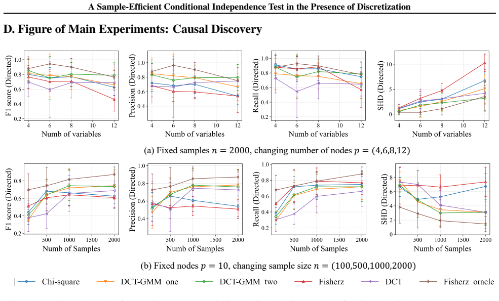
- [Section 4.1 and Figure 2] The text says the first two columns of Figure 2 show Type I error, but the caption refers to all four columns as 'Type I and Type II error (1-power)'. Please label each panel clearly so the reader can map columns to the two experimental designs.
- [Appendix F.4.2, final display] The final display writes the limit distribution as Φ(·) without the √n scaling, and with 1/n^2 inside the variance; this is inconsistent with Theorem 3.4 and should be corrected as part of the scaling fix described in the major comments.
Circularity Check
No significant circularity; the GMM covariance estimator is a standard application of Hansen's (1982) GMM theory under an explicitly stated Gaussian-copula model, and the load-bearing self-citation (DCT's Theorem 3.4) is independently published with its proof reproduced in the appendix.
full rationale
The derivation chain walks from an explicitly stated model to the test without any step that defines its target in terms of its own output. The latent-Gaussian assumption (Section 3, Problem Setting, Eq. 1) is an input, and Appendix B openly acknowledges its restrictiveness; that is weighed here as an honest limitation, not a circular move. The moment functions in Eq. (4) are validated in Appendix F.1 by showing E[f_i(θ*)] = 0 follows from the model's own cell-probability formula (Eq. 3), so the moment conditions are consequences of the stated model, and the CI conclusion is a function of the estimated covariance rather than the reverse. Asymptotic normality of the GMM estimator (Theorem 3.1, Lemma 3.2) is external Hansen (1982) GMM theory, with derivations in F.2 and F.3. The nodewise-regression link (Lemma 3.3, Theorem 3.4) is taken from the authors' own prior DCT paper; Section 3.2 says 'we follow (Sun et al., 2024)', and Appendix F.4 states 'the following proof is a direct copy from (Sun et al., 2024)' before reproducing the proof, which rests on external nodewise-regression results (Callot et al., 2019). This self-citation is load-bearing for the CI-test construction, but it is independently published (arXiv:2404.17644), reproduced in full in the appendix, and its assumptions do not include the present test's validity, so under the review rules it is real evidence and does not by itself raise the circularity score. The variance-superiority claim (Theorem 3.5, Appendix G) is a direct algebraic identity (a just-identified GMM with A = S^-1 has variance G^-1 S G^-T, equal to DCT's Z-estimator variance) plus the classical GMM efficiency gain from adding valid moment conditions. Two correctness risks are flagged and kept out of the circularity score: Theorem 3.1 Eq. (6) and Lemma 3.2 Eq. (7) write √n(σ̂−σ*) = −(1/n)Σ[...], mixing an O_p(1) left side with an O_p(n^-1/2) right side (the proof in F.2 derives the unscaled form), and Algorithms 1-2 compute p = 2(1−Φ(|β̂|)) at Step 16/18 without the √(V/n) normalization required by Theorem 3.4, which as written would not control Type I error. A scholarship gap is also noted without scoring it as circularity: the cell-probability threshold-estimation construction is classical polychoric correlation, which the paper does not cite (e.g., Olsson 1979). Overall the central GMM claim has independent content and is not forced by self-citation or by construction, so the score is 1.
Assumptions & free parameters
assumptions (4)
- domain assumption The latent continuous variables X follow a zero-mean unit-variance multivariate normal distribution (Gaussian copula after unknown monotone transformations).
- domain assumption Each observable discrete variable arises by applying an unknown monotone function and then thresholding the latent variable (nonparanormal discretization).
- standard math Standard GMM regularity conditions hold: differentiability of moment functions, interior optimum, consistent variance estimator.
- domain assumption For causal discovery, the causal Markov condition and faithfulness hold.
Cite this review
Pith. "Pith review of A Sample Efficient Conditional Independence Test in the Presence of Discretization." pith.science (2026). https://pith.science/paper/3IS3GM33
@misc{pith2026250608747,
  author       = {Pith},
  title        = {Pith review of: A Sample Efficient Conditional Independence Test in the Presence of Discretization},
  year         = {2026},
  howpublished = {\url{https://pith.science/paper/3IS3GM33}},
  note         = {Machine review of arXiv:2506.08747}
}
read the original abstract
In many real-world scenarios, interested variables are often represented as discretized values due to measurement limitations. Applying Conditional Independence (CI) tests directly to such discretized data, however, can lead to incorrect conclusions. To address this, recent advancements have sought to infer the correct CI relationship between the latent variables through binarizing observed data. However, this process inevitably results in a loss of information, which degrades the test's performance. Motivated by this, this paper introduces a sample-efficient CI test that does not rely on the binarization process. We find that the independence relationships of latent continuous variables can be established by addressing an over-identifying restriction problem with Generalized Method of Moments (GMM). Based on this insight, we derive an appropriate test statistic and establish its asymptotic distribution correctly reflecting CI by leveraging nodewise regression. Theoretical findings and Empirical results across various datasets demonstrate that the superiority and effectiveness of our proposed test. Our code implementation is provided in https://github.com/boyangaaaaa/DCT
Figures


Figures from the paper (4 more)



Reference graph
Works this paper leans on
-
[1]
F., Statnikov, A., Tsamardinos, I., Mani, S., and Koutsoukos, X
Aliferis, C. F., Statnikov, A., Tsamardinos, I., Mani, S., and Koutsoukos, X. D. Local causal and markov blanket induction for causal discovery and feature selection for classification part i: algorithms and empirical evaluation. Journal of Machine Learning Research, 11 0 (1), 2010
work page 2010
-
[2]
Asratian, A. S., Denley, T. M., and H \"a ggkvist, R. Bipartite graphs and their applications, volume 131. Cambridge university press, 1998
work page 1998
-
[3]
Partial correlation and conditional correlation as measures of conditional independence
Baba, K., Shibata, R., and Sibuya, M. Partial correlation and conditional correlation as measures of conditional independence. Australian & New Zealand Journal of Statistics, 46 0 (4): 0 657--664, 2004
work page 2004
-
[4]
A nodewise regression approach to estimating large portfolios, 2019
Callot, L., Caner, M., Ulasan, E., and Özlem Önder, A. A nodewise regression approach to estimating large portfolios, 2019
work page 2019
-
[5]
causaldag : creation, manipulation, and learning of causal models , 2018
Chandler Squires . causaldag : creation, manipulation, and learning of causal models , 2018. URL https://github.com/uhlerlab/causaldag
work page 2018
-
[6]
Changsheng, H. and Yongfeng, W. Investor sentiment and assets valuation. Systems Engineering Procedia, 3: 0 166--171, 2012
work page 2012
-
[7]
Investment valuation: Tools and techniques for determining the value of any asset, volume 666
Damodaran, A. Investment valuation: Tools and techniques for determining the value of any asset, volume 666. John Wiley & Sons, 2012
work page 2012
-
[8]
A versatile causal discovery framework to allow causally-related hidden variables
Dong, X., Huang, B., Ng, I., Song, X., Zheng, Y., Jin, S., Legaspi, R., Spirtes, P., and Zhang, K. A versatile causal discovery framework to allow causally-related hidden variables. In ICLR, 2024 a
work page 2024
Show all 36 references
-
[9]
On the parameter identifiability of partially observed linear causal models
Dong, X., Ng, I., Huang, B., Sun, Y., Jin, S., Legaspi, R., Spirtes, P., and Zhang, K. On the parameter identifiability of partially observed linear causal models. In NeurIPS, 2024 b
2024
-
[10]
Permutation-based rank test in the presence of discretization and application in causal discovery with mixed data
Dong, X., Ng, I., Sun, B., Dai, H., Hao, G.-Y., Fan, S., Spirtes, P., Qiu, Y., and Zhang, K. Permutation-based rank test in the presence of discretization and application in causal discovery with mixed data. In ICML, 2025
2025
-
[11]
Movietweetings: a movie rating dataset collected from twitter
Dooms, S., De Pessemier, T., and Martens, L. Movietweetings: a movie rating dataset collected from twitter. In Workshop on Crowdsourcing and human computation for recommender systems, CrowdRec at RecSys, volume 2013, pp.\ 43, 2013
2013
-
[12]
and Tarsi, M
Dor, D. and Tarsi, M. A simple algorithm to construct a consistent extension of a partially oriented graph. 1992. URL https://api.semanticscholar.org/CorpusID:122949140
1992
-
[13]
A permutation-based kernel conditional independence test
Doran, G., Muandet, K., Zhang, K., and Sch \"o lkopf, B. A permutation-based kernel conditional independence test. In UAI, pp.\ 132--141, 2014
2014
-
[14]
Probable Error
Fisher, R. A. On the " Probable Error " of a Coefficient of Correlation Deduced from a Small Sample . Metron, 1: 0 3--32, 1921
1921
-
[15]
F.R.S., K. P. X. on the criterion that a given system of deviations from the probable in the case of a correlated system of variables is such that it can be reasonably supposed to have arisen from random sampling. Philosophical Magazine Series 1, 50: 0 157--175, 2009. URL http...
2009
-
[16]
R., and Jordan, M
Fukumizu, K., Bach, F. R., and Jordan, M. I. Dimensionality reduction for supervised learning with reproducing kernel hilbert spaces. Journal of Machine Learning Research, 5 0 (Jan): 0 73--99, 2004
2004
-
[17]
Hansen, L. P. Large sample properties of generalized method of moments estimators. Econometrica, 50 0 (4): 0 1029--1054, 1982. ISSN 00129682, 14680262. URL http://www.jstor.org/stable/1912775
1982
-
[18]
U., Ulvenes, P
Johnson, S. U., Ulvenes, P. G., ktedalen, T., and Hoffart, A. Psychometric properties of the general anxiety disorder 7-item (gad-7) scale in a heterogeneous psychiatric sample. Frontiers in psychology, 10: 0 449461, 2019
2019
-
[19]
How to gain on power: Novel conditional independence tests based on short expansion of conditional mutual information
Kubkowski, M., Mielniczuk, J., and Teisseyre, P. How to gain on power: Novel conditional independence tests based on short expansion of conditional mutual information. Journal of Machine Learning Research, 22 0 (62): 0 1--57, 2021. URL http://jmlr.org/papers/v22/19-600.html
2021
-
[20]
McDonald, J. H. Handbook of biological statistics, volume 2. sparky house publishing Baltimore, MD, 2009
2009
-
[21]
Structured learning of gaussian graphical models
Mohan, K., Chung, M., Han, S., Witten, D., Lee, S.-I., and Fazel, M. Structured learning of gaussian graphical models. Advances in neural information processing systems, 25, 2012
2012
-
[22]
A., Luft, M
Mossman, S. A., Luft, M. J., Schroeder, H. K., Varney, S. T., Fleck, D. E., Barzman, D. H., Gilman, R., DelBello, M. P., and Strawn, J. R. The generalized anxiety disorder 7-item (gad-7) scale in adolescents with generalized anxiety disorder: signal detection and validation. A...
2017
-
[23]
Newey, W. K. Generalized method of moments. Access through internet: https://ocw. mit. edu/courses/economics/14-386-new-econometric-methods-spring-2007/readings/ngmm07. pdf, 2007
2007
-
[24]
Causality: Models, Reasoning, and Inference
Pearl, J. Causality: Models, Reasoning, and Inference . Cambridge University Press, 2000. ISBN 0521773628. URL http://www.worldcat.org/isbn/0521773628
2000
-
[25]
C., and Vannucci, M
Peterson, C., Stingo, F. C., and Vannucci, M. Bayesian inference of multiple gaussian graphical models. Journal of the American Statistical Association, 110 0 (509): 0 159--174, 2015
2015
-
[26]
Ren, Z., Sun, T., Zhang, C.-H., and Zhou, H. H. Asymptotic normality and optimalities in estimation of large gaussian graphical models. 2015
2015
-
[27]
Sparling, E. I. and Sen, S. Rating: how difficult is it? In Proceedings of the fifth ACM conference on Recommender systems, pp.\ 149--156, 2011
2011
-
[28]
Causation, Prediction, and Search
Spirtes, P., Glymour, C., and Scheines, R. Causation, Prediction, and Search. MIT press, 2nd edition, 2000
2000
-
[29]
V., Zhang, K., and Visweswaran, S
Strobl, E. V., Zhang, K., and Visweswaran, S. Approximate kernel-based conditional independence tests for fast non-parametric causal discovery. Journal of Causal Inference, 7 0 (1): 0 20180017, 2019
2019
-
[30]
A conditional independence test in the presence of discretization, 2024
Sun, B., Yao, Y., Hao, H., Qiu, Y., and Zhang, K. A conditional independence test in the presence of discretization, 2024. URL https://arxiv.org/abs/2404.17644
2024 arXiv
-
[31]
Vaart, A. W. v. d. M–and Z-Estimators, pp.\ 41–84. Cambridge Series in Statistical and Probabilistic Mathematics. Cambridge University Press, 1998. doi:10.1017/CBO9780511802256.006
1998 doi
-
[32]
and Lin, Y
Yuan, M. and Lin, Y. Model selection and estimation in the gaussian graphical model. Biometrika, 94 0 (1): 0 19--35, 2007
2007
-
[33]
Kernel-based conditional independence test and application in causal discovery
Zhang, K., Peters, J., Janzing, D., and Sch \"o lkopf, B. Kernel-based conditional independence test and application in causal discovery. arXiv preprint arXiv:1202.3775, 2012
2012 arXiv
-
[34]
An improved iamb algorithm for markov blanket discovery
Zhang, Y., Zhang, Z., Liu, K., and Qian, G. An improved iamb algorithm for markov blanket discovery. J. Comput., 5 0 (11): 0 1755--1761, 2010
2010
-
[35]
Ziegel, E. R. Statistical inference, 2002
2002
-
[36]
write newline
" write newline "" before.all 'output.state := FUNCTION n.dashify 't := "" t empty not t #1 #1 substring "-" = t #1 #2 substring "--" = not "--" * t #2 global.max substring 't := t #1 #1 substring "-" = "-" * t #2 global.max substring 't := while if t #1 #1 substring * t #2 gl...
Reviewed August 7, 2026 · model on record in the stance chip above.
Discussion (0). Sign in to comment.