REVIEW 3 major objections 5 minor 55 references
Nonlinear Splitting for Gradient-Based Unconstrained and Adjoint Optimization
T0 review · 3 major / 5 minor · reviewed 2026-08-15 · deepseek-v4-flash
Pith's one-line read Nonlinear splitting—replacing a gradient or constraint by a two-argument function that agrees on the diagonal—turns explicit gradient methods into semi-implicit ones stable at large step sizes and, in a neutron transport test, needs one…
desk verdict A promising nonlinear splitting framework whose constrained-case Algorithm 1 does not follow from the paper's own derivation; the unconstrained part is cleaner and the paper deserves refereeing but needs real fixing. read the letter →
The pith
A machine-rendered reading of the paper's core claim, the machinery that carries it, and where it could break.
The reading
What carries the argument
The load-bearing object is the nonlinear splitting: a smooth two-argument function $g(x,y)$ that coincides with the original function on the diagonal, $g(x,x)=f(x)$. Applied to gradients, it turns explicit descent into the semi-implicit NS-GD step; applied to the equality constraint, it yields $\widetilde{F}(x,y;\theta)$ with $\widetilde{F}(x,x;\theta)=F(x;\theta)$, and the induced split gradient is defined through a modified adjoint system. The paper's main constructive device is the single iteration of a fixed-point solver: writing $x_{k+1}=G(x_k;\theta_k)$ and setting $\widetilde{F}(x,y;\theta)=G(x;\theta)-y$ converts any existing nonlinear solver into a constraint splitting, so the adjoint can be evaluated at a state that does not yet satisfy the constraint. A secondary device is the linearly-implicit gradient splitting $\widetilde{\nabla C}(x,y)=L(x)y+g(x)$, which makes each NS-GD step one linear solve, and the one-step linearized version of the implicit update, which produces a preconditioned gradient method with preconditioner determined by the splitting. These two devices together carry the reported gains in stability and in reduced solver work.
What would settle it
For the scalar problem $\min_\theta (x-\theta)^2$ subject to $x=\theta$, take the solver iteration $G(x;\theta)=x+2(\theta-x)$, which has the correct fixed point $\theta$ but overshoots on every step. Applying Algorithm 1 at a state $x\neq\theta$ and checking whether the split-gradient direction $\widetilde{\nabla_\theta J}(\theta)[x,G(x;\theta)]$ has negative inner product with $\theta-\theta^*$ settles the descent question directly: if that inner product is positive for any $\theta$, the central premise of the constrained construction fails. This one-dimensional calculation can be done by hand.
Extended reading notes
Core claim
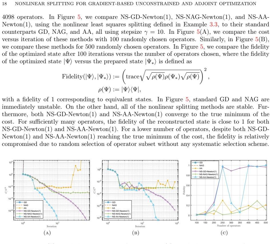
The central discovery, stated as a construction, is that evaluating a gradient or an equality constraint on two arguments instead of one splits the original object and yields a family of semi-implicit optimization methods. In the unconstrained case, a nonlinearly split gradient $\widetilde{\nabla C}(x,y)$ with diagonal value $\nabla C(x)$ gives the NS-GD update (3.2); when the splitting has the linearly-implicit form $L(x)y+g(x)$, each step is a single linear solve. A single linearized solve of the implicit step produces a preconditioned gradient descent whose preconditioner is determined by the chosen splitting, and for nonlinear least squares the split gradient $J(x)^\top r(y)$ recovers the classical damped least-squares update as a special case. In the equality-constrained case, any nonlinear solver written as $x_{k+1}=G(x_k;\theta_k)$ defines a constraint splitting $\widetilde{F}(x,y;\theta)=G(x;\theta)-y$; using one solver iteration as the state update and solving a modified adjoint equation gives a split gradient that is consistent with the true adjoint gradient when $x_{k+1}$ actually solves the constraint. The paper demonstrates numerically that these methods take larger stable steps on three two-dimensional nonconvex benchmark functions, stabilize and converge in a 128-real-dimensional quantum tomography least-squares problem, reduce forward transport solves by a factor of two to three in the neutron transport example, and add a momentum-like term to the initial condition of an ODE-constrained problem that prevents divergence at large step size.
Load-bearing premise
The load-bearing premise is that a single iteration of a nonlinear solver leaves the state slightly off the constraint yet still produces a split gradient that points downhill, so that updating the parameters along that direction decreases the objective; the paper gives no descent or convergence theorem for this, and Section 5 explicitly defers stability and convergence analysis.
Editorial extensions
If this is right
- NS-GD and its momentum-accelerated variant remain stable at step sizes where explicit gradient and momentum methods diverge, allowing the iterates on nonconvex benchmark problems to escape local minima and reach the global minimum.
- For nonlinear least squares, the split gradient $\widetilde{\nabla C}(x,y)=J(x)^\top r(y)$ turns the one-linearized-solve variant of NS-GD into the classical damped least-squares update, and the fixed-point-accelerated version converges where standard gradient methods diverge at step size $\gamma=10$.
- In adjoint-based optimization, one nonlinear-solver iteration per optimization step is enough to produce a usable split gradient; the neutron transport experiments reach the same objective and constraint residual with two to three times fewer forward transport solves than adjoint methods that solve the constraint to tolerance $10^{-6}$ each step.
- Splitting the equality constraint of an initial-value problem adds a momentum-like term to the initial condition, and the example shows that the resulting method ($\alpha=0.5$ or $1$) reaches the minimum at a step size that destabilizes the standard method ($\alpha=0$).
- Both momentum and fixed-point acceleration compose with the nonlinear splitting construction, and the paper reports that the accelerated variants match or beat their standard counterparts in objective and runtime on the tested problems.
Reading between the lines
- Editorial inference: If a broad descent condition can be proven for split gradients—for example, a monotonicity assumption that generalizes the mean-value property already known to make discrete gradients descent directions—then the construction would unify proximal gradient, damped least-squares, preconditioned gradient descent, and adjoint methods as instances of one recipe.
- Editorial inference: The constraint-splitting recipe is transferable: any optimization loop that already contains a fixed-point solver for the state equation can switch to one-solver-iteration state updates and a modified adjoint, converting solver iterations into optimization progress. The neutron transport result suggests this can be tested in other expensive implicit-constraint settings, where
- Editorial inference: The diagonal condition $\widetilde{\nabla C}(x,x)=\nabla C(x)$ is only consistency; all of the reported stability must come from off-diagonal behavior of the chosen splitting. A natural testable extension is to design splittings whose off-diagonal term equals a desired preconditioner, or a quadratic surrogate whose minimizer is the global minimizer, which the benchmark results
- Editorial inference: Since the paper's theory is deferred, the safest reading is that the framework is a method generator whose effectiveness is demonstrated empirically on a handful of problems; the factor-three solve reduction is a single experiment, not yet a theorem, so a broader benchmark across initial conditions and problem scales would determine how general the gain is.
Signed reviews
Editorial analysis
A structured set of objections, weighed in public.
Referee Report
Summary. The paper proposes a nonlinear splitting framework for gradient-based optimization. For unconstrained problems, it defines a splitting of the gradient as a function g(x,y) with g(x,x)=∇C(x), leading to semi-implicit gradient methods and accelerated variants (NS-GD, NS-NAG, NS-GD-Newton(1), NS-NAG-Newton(1), NS-AA-Newton(1)). For equality-constrained problems, it splits the constraint F(x,θ) and uses a modified adjoint to compute a 'split gradient' that does not require solving the constraint exactly, yielding algorithms NS-Adj-GD, NS-Adj-NAG, and NS-Adj-AA. Numerical experiments on nonconvex benchmark functions, quantum tomography, neutron transport source optimization, and an ODE-constrained problem demonstrate improved stability, large-step capability, and, in the transport example, a claimed reduction of high-dimensional kinetic solves by up to a factor of three compared with standard adjoint optimization.
Significance. If correct, the framework provides a general and potentially useful construction for semi-implicit gradient methods and inexact-adjoint optimization. The unconstrained part is elegant: it unifies existing methods such as proximal gradient and Levenberg–Marquardt as special cases, connects to discrete gradient methods, and the empirical large-step stability on nonconvex benchmarks is striking. The constrained part addresses a practically important bottleneck in PDE-constrained optimization. However, the significance is tempered by the absence of descent or convergence analysis, which the paper itself defers, and by an internal inconsistency between the derived modified adjoint and the algorithm used in the constrained-case experiments. These issues undermine the claimed factor-of-three result as a validation of the proposed systematic construction.
major comments (3)
- [§3.2, Eqs. (3.25)–(3.27) and Algorithm 1] The modified adjoint construction applied to the splitting eF(x,y;θ)=G(x;θ)−y yields the adjoint equation (D1G(x_k;θ_k)−I)^*λ = −∂J(x_{k+1})/∂x and the split gradient ∂J/∂θ + ⟨λ, ∂G(x_k;θ_k)/∂θ⟩. Algorithm 1 instead states D1F(x_{k+1};θ_k)^*λ = −∂J(x_{k+1})/∂x and ∂F(x_{k+1};θ_k)/∂θ, which, with F(x;θ)=G(x;θ)−x, means evaluating D1G and ∂G/∂θ at x_{k+1} rather than x_k. These expressions agree only if G is affine in its state argument. For the linearized neutron transport map of §4.2.1, G depends on ψ_k through φ_k in the scattering cross-section, so that condition fails. Consequently, the algorithm whose numerical results are reported in §4.2.1 is not the split gradient derived in §3.2; it is a heuristic standard-adjoint evaluation at an inexact state. This disconnect directly affects the factor-of-three claim in the abstract.
- [§5 and §3.2] No descent or convergence analysis is provided for any of the proposed methods. For NS-GD, the discrete-gradient property (Example 3.2) guarantees monotonic decrease only when the splitting satisfies the mean-value condition (3.6), which the linearly-implicit splittings of §4.1.1 do not. For NS-Adj-GD, e∇θJ is not the true gradient of the reduced objective when x_{k+1}≠x_k, and there is no guarantee that the update θ_{k+1}=θ_k−γe∇θJ decreases J. The paper explicitly defers this analysis to future work in Section 5. Given that the central claim is improved accuracy and efficiency, the absence of even a local descent result leaves the empirical gains unexplained and limits the generality of the proposed framework.
- [§3.2, discussion after Eq. (3.26)] The statement that 'the term ∂F/∂θ depending on both x_k and x_{k+1}' is inaccurate: for the splitting eF(x,y;θ)=G(x;θ)−y, the partial derivative with respect to θ depends only on the first argument x_k. This confusion appears to stem from conflating the original constraint with the fixed-point residual F(x;θ)=G(x;θ)−x. Please clarify which operator is used in (3.26b)–(3.26c) and whether the modified adjoint is derived from the splitting eF or from the redefined constraint F.
minor comments (5)
- [Abstract and §4.2.1] The abstract states that the total number of kinetic solves is reduced by a factor of three, while Figure 6(B) and the text report '2−3× less'; please make the quantitative claim consistent.
- [§4.1.1, Rastrigin splitting] The Rastrigin splitting contains factors y_i/x_i, which are undefined at x_i=0. Please specify the treatment of this singularity or restrict the initial conditions to avoid it.
- [§4.1.2] The text '46 = 4098' should read 4^6 = 4096; correspondingly, the number of Pauli operators is 4096, not 4098.
- [Table 2] The runtime comparison with MATLAB built-in optimizers is difficult to interpret because the NS methods are implemented in unoptimized MATLAB loops while the built-ins are compiled; the authors acknowledge this in the text, but a caveat in the table caption would be helpful.
- [§3.1] The statement that a closed one-form on R^N has an associated cost function is true but could be stated more precisely, e.g., 'on a simply connected domain, a closed one-form is exact'.
Circularity Check
No significant circularity: the nonlinear-splitting framework is defined in-paper and tested against external benchmarks; the flagged Algorithm 1 derivative mismatch is a correctness gap, not a circular reduction.
full rationale
The paper's central unconstrained and constrained constructions are self-contained. Definitions 3.1-3.3 define nonlinear splittings of gradients and equality constraints in terms of the diagonal consistency condition g(x,x)=f(x), and the modified-adjoint construction (3.27a-c) is verified by direct reduction to the standard adjoint when x=y. This is an internal consistency check, not a prediction that was assumed. The numerical claims are supported by external comparisons: MATLAB built-in optimizers for the benchmark nonconvex functions, standard GD/NAG/AA in the quantum tomography problem, and standard adjoint methods in the neutron-transport example, where the target state is generated by a known forward solve rather than fitted to the proposed method. Self-citations to the authors' earlier time-integration work on nonlinear splitting (e.g., [15, 51, 45, 46, 50, 52]) motivate the ansatz but are not load-bearing; the optimization framework is derived in this paper and stands on its own equations. Section 5 explicitly defers convergence and stability analysis; that is a missing-theory limitation, which per the scoring rules belongs to correctness risk rather than circularity. One non-circular technical caveat should be flagged: Algorithm 1 evaluates D1F(x_{k+1};theta_k) and partial F(x_{k+1};theta_k)/partial theta, whereas the general formula (3.27a-c) applied to eF(x,y;theta)=G(x;theta)-y requires the derivatives at x_k, namely DG(x_k)-I and partial G(x_k)/partial theta. In the state-dependent transport example these differ, so the implemented constrained-case algorithm is not exactly the paper's derived split gradient. This is an internal-consistency and correctness concern, not an input-output circularity, so it does not raise the circularity score beyond 2.
Assumptions & free parameters
free parameters (6)
- stepsize gamma for unconstrained benchmarks =
0.1
- stepsize gamma for quantum tomography =
10
- stepsize gamma for neutron transport =
5e-9
- momentum factor mu for NAG variants =
0.9 for neutron transport
- Anderson acceleration depth m =
25 for neutron transport
- momentum coefficient alpha in the IVP example =
0, 0.5, 1
assumptions (5)
- domain assumption The objective C is C^1 and its gradient has a differentiable two-argument splitting.
- domain assumption A parameter-to-state map x[theta] exists and is differentiable, as needed for the standard adjoint gradient.
- domain assumption Fixed points of the nonlinear solver G correspond to solutions of the equality constraint F=0.
- ad hoc to paper The handcrafted linearly-implicit splittings for the benchmark functions are valid and stable on the iterates.
- ad hoc to paper The split gradient is a descent direction even when x and y differ.
Cite this review
Pith. "Pith review of Nonlinear Splitting for Gradient-Based Unconstrained and Adjoint Optimization." pith.science (2026). https://pith.science/paper/3UT27TLH
@misc{pith2026250820280,
  author       = {Pith},
  title        = {Pith review of: Nonlinear Splitting for Gradient-Based Unconstrained and Adjoint Optimization},
  year         = {2026},
  howpublished = {\url{https://pith.science/paper/3UT27TLH}},
  note         = {Machine review of arXiv:2508.20280}
}
abstract
High dimensional and/or nonconvex optimization remains a challenging and important problem across a wide range of fields, such as machine learning, data assimilation, and partial differential equation (PDE) constrained optimization. Here we consider gradient-based methods for solving unconstrained and constrained optimization problems, and introduce the concept of nonlinear splitting to improve accuracy and efficiency. For unconstrained optimization, we consider splittings of the gradient to depend on two arguments, leading to semi-implicit gradient optimization algorithms. In the context of adjoint-based constrained optimization, we propose a splitting of the constraint $F(\mathbf{x},\theta)$, effectively expanding the space on which we can evaluate the ``gradient''. In both cases, the formalism further allows natural coupling of nonlinearly split optimization methods with acceleration techniques, such as Nesterov or Anderson acceleration. The framework is demonstrated to outperform existing methods in terms of accuracy and/or runtime on a handful of diverse optimization problems. This includes low-dimensional analytic nonconvex functions, high-dimensional nonlinear least squares in quantum tomography, and PDE-constrained optimization of kinetic equations, where the total number of high-dimensional kinetic solves is reduced by a factor of three compared with standard adjoint optimization.
Figures


Figures from the paper (6 more)



Reference graph
Works this paper leans on
-
[1]
James P. Abbott and Richard P. Brent. Fast local convergence with single and multistep methods for nonlinear equations.The Journal of the Australian Mathematical Society. Series B. Applied Mathematics, 19(2):173–199, 1975. (Page 3)
work page 1975
-
[2]
Filippo Aluffi-Pentini, Valerio Parisi, and Francesco Zirilli. A differential-equations algorithm for nonlinear equations.ACM Transactions on Mathematical Software (TOMS), 10(3):299–316,
-
[3]
On the Minimizing Property of a Second Order Dissipative System in Hilbert Spaces
Felipe Alvarez. On the Minimizing Property of a Second Order Dissipative System in Hilbert Spaces. SIAM Journal on Control and Optimization, 38(4):1102–1119, 2000. (Page 4)
work page 2000
-
[4]
Natural gradient works efficiently in learning.Neural computation, 10(2):251– 276, 1998
Shun-Ichi Amari. Natural gradient works efficiently in learning.Neural computation, 10(2):251– 276, 1998. (Page 3)
work page 1998
-
[5]
R. Anderson, J. Andrej, A. Barker, J. Bramwell, J.-S. Camier, J. Cerveny, V. Dobrev, Y. Du- douit, A. Fisher, Tz. Kolev, W. Pazner, M. Stowell, V. Tomov, I. Akkerman, J. Dahm, D. Med- ina, and S. Zampini. MFEM: A modular finite element methods library.Computers & Mathe- matics with Applications, 81:42–74, 2021. (Page 19)
work page 2021
-
[6]
Uri M Ascher, Steven J Ruuth, and Brian TR Wetton. Implicit-explicit methods for time- dependent partial differential equations.SIAM Journal on Numerical Analysis, 32(3):797–823,
-
[7]
H. Attouch, X. Goudou, and P. Redont. The heavy ball with friction method, i. the con- tinuous dynamical system: Global exploration of the local minima of a real-valued function by asymptotic analysis of a dissipative dynamical system.Communications in Contemporary Mathematics, 2(01):1–34, 2000. (Page 4)
work page 2000
-
[8]
Guillaume Bal, Francis J. Chung, and John C. Schotland. Ultrasound modulated biolumines- cence tomography and controllability of the radiative transport equation.SIAM Journal on Mathematical Analysis, 48(2):1332–1347, 2016. (Page 18)
work page 2016
Show all 55 references
-
[9]
Bertsekas.Constrained Optimization and Lagrange Multiplier Methods
Dimitri P. Bertsekas.Constrained Optimization and Lagrange Multiplier Methods. Academic Press, 1982. (Page 9)
1982
-
[10]
LinearlyImplicitIMEXRunge– Kutta Methods for a Class of Degenerate Convection-Diffusion Problems.SIAM Journal on Scientific Computing, 37(2):B305–B331, 2015
S.Boscarino, R.Bürger, P.Mulet, G.Russo, andL.M.Villada. LinearlyImplicitIMEXRunge– Kutta Methods for a Class of Degenerate Convection-Diffusion Problems.SIAM Journal on Scientific Computing, 37(2):B305–B331, 2015. (Page 6)
2015
-
[11]
Boscarino, F
S. Boscarino, F. Filbet, and G. Russo. High Order Semi-implicit Schemes for Time Dependent Partial Differential Equations. Journal of Scientific Computing, 68(3):975–1001, 2016. (Page 5)
2016
-
[12]
Differential gradient methods
C.A Botsaris. Differential gradient methods. Journal of Mathematical Analysis and Applica- tions, 63(1):177–198, 1978. (Page 3)
1978
-
[13]
A. A. Brown and M. C. Bartholomew-Biggs. Some effective methods for unconstrained op- timization based on the solution of systems of ordinary differential equations. Journal of Optimization Theory and Applications, 62(2):211–224, 1989. (Page 4)
1989
-
[14]
Brune, Matthew G
Peter R. Brune, Matthew G. Knepley, Barry F. Smith, and Xuemin Tu. Composing scalable nonlinear algebraic solvers.SIAM Review, 57(4):535–565, 2015. (Page 11) 26 NONLINEAR SPLITTING FOR GRADIENT-BASED UNCONSTRAINED AND ADJOINT OPTIMIZATION
2015
-
[15]
Buvoli and B
T. Buvoli and B. S. Southworth. A new class of Runge–Kutta methods for nonlinearly parti- tioned systems. arXiv preprint: 2401.04859, 2023. (Page 5)
2023 arXiv
-
[16]
Calvo, J
M.P. Calvo, J. de Frutos, and J. Novo. Linearly implicit Runge–Kutta methods for advec- tion–reaction–diffusion equations.Applied Numerical Mathematics, 37(4):535–549, 2001. (Page 6)
2001
-
[17]
Woodhead Publishing Series in Energy
Liangzhi Cao and Hongchun Wu, editors.Deterministic Numerical Methods for Unstructured- Mesh Neutron Transport Calculation. Woodhead Publishing Series in Energy. Woodhead Pub- lishing, 2021. (Page 19)
2021
-
[18]
Iterativepre-conditioningtoexpedite the gradient-descent method
KushalChakrabarti, NirupamGupta, andNikhilChopra. Iterativepre-conditioningtoexpedite the gradient-descent method. In2020 American Control Conference (ACC), pages 3977–3982,
-
[19]
Alvarez D
F. Alvarez D. and J. M. Pérez C. A Dynamical System Associated with Newton’s Method for Parametric Approximations of Convex Minimization Problems.Applied Mathematics and Optimization, 38(2):193–217, 1998. (Page 3)
1998
-
[20]
A geometric integration approach to smooth optimization: foundations of the discrete gradient method
Matthias J Ehrhardt, Erlend S Riis, Torbjørn Ringholm, and Carola-Bibiane Schönlieb. A geometric integration approach to smooth optimization: foundations of the discrete gradient method. IMA Journal of Numerical Analysis, 45(3):1269–1299, 2024. (Page 6, 7)
2024
-
[21]
M. B. Giles and N. A. Pierce. An introduction to the adjoint approach to design. Flow, Turbulence and Combustion, 65:393–415, 2000. (Page 9)
2000
-
[22]
Giles and Endre Süli
Michael B. Giles and Endre Süli. Adjoint methods for PDEs: a posteriori error analysis and postprocessing by duality.Acta Numerica, 11:145–236, 2002. (Page 9)
2002
-
[23]
An inverse source problem in radiative transfer with partial data.Inverse Problems, 27(12):125009, 2011
Mark Hubenthal. An inverse source problem in radiative transfer with partial data.Inverse Problems, 27(12):125009, 2011. (Page 18)
2011
-
[24]
Matlab version: R2024a, 2024
The MathWorks Inc. Matlab version: R2024a, 2024. (Page 14)
2024
-
[25]
A New Method for Solving Nonlinear Simultaneous Equations.SIAM Journal on Numerical Analysis, 16(5):779–789, 1979
Sandro Incerti, Valerio Parisi, and Francesco Zirilli. A New Method for Solving Nonlinear Simultaneous Equations.SIAM Journal on Numerical Analysis, 16(5):779–789, 1979. (Page 4)
1979
-
[26]
An Almost-Linear- Time Algorithm for Approximate Max Flow in Undirected Graphs, and its Multicommodity Generalizations
Jonathan A Kelner, Yin Tat Lee, Lorenzo Orecchia, and Aaron Sidford. An Almost-Linear- Time Algorithm for Approximate Max Flow in Undirected Graphs, and its Multicommodity Generalizations. arXiv, 2013. (Page 3)
2013
-
[27]
Kulkarni, David M
Mandar D. Kulkarni, David M. Cross, and Robert A. Canfield. Discrete adjoint formulation for continuum sensitivity analysis.AIAA Journal, 54(2):758–766, 2016. (Page 9)
2016
-
[28]
A grey transport acceleration method far time-dependent radiative transfer problems
Edward Larsen. A grey transport acceleration method far time-dependent radiative transfer problems. Journal of Computational Physics, 78(2):459–480, 1988. (Page 5)
1988
-
[29]
Rabelo, Dirk A
Antonio Leitão, Joel C. Rabelo, Dirk A. Lorenz, and Maximilian Winkler. On inertial Levenberg-Marquardt type methods for solving nonlinear ill-posed operator equations.arXiv preprint:2406.07044, 2024. (Page 9)
2024 arXiv
-
[30]
A method for the solution of certain non-linear problems in least squares
Kenneth Levenberg. A method for the solution of certain non-linear problems in least squares. Quart. Appl. Math., 2:164–168, 1944. (Page 8)
1944
-
[31]
Li and L
S. Li and L. Petzold. Adjoint sensitivity analysis for time-dependent partial differential equa- tions with adaptive mesh refinement.Journal of Computational Physics, 198(1):310–325, 2004. (Page 9)
2004
-
[32]
Preconditioned stochastic gradient descent.IEEE Transactions on Neural Networks and Learning Systems, 29(5):1454–1466, 2018
Xi-Lin Li. Preconditioned stochastic gradient descent.IEEE Transactions on Neural Networks and Learning Systems, 29(5):1454–1466, 2018. (Page 3)
2018
-
[33]
From differential equation solvers to accelerated first-order methods for convex optimization.Mathematical Programming, 195(1-2):735–781, 2022
Hao Luo and Long Chen. From differential equation solvers to accelerated first-order methods for convex optimization.Mathematical Programming, 195(1-2):735–781, 2022. (Page 4)
2022
-
[34]
Maddison, Daniel Paulin, Yee Whye Teh, and Arnaud Doucet
Chris J. Maddison, Daniel Paulin, Yee Whye Teh, and Arnaud Doucet. Dual space precondi- tioning for gradient descent.SIAM Journal on Optimization, 31(1):991–1016, 2021. (Page 3, 7) NONLINEAR SPLITTING FOR GRADIENT-BASED UNCONSTRAINED AND ADJOINT OPTIMIZATION 27
2021
-
[35]
Marquardt
Donald W. Marquardt. An algorithm for least-squares estimation of nonlinear parameters. Journal of the Society for Industrial and Applied Mathematics, 11(2):431–441, 1963. (Page 8)
1963
-
[36]
(Page 19)
MFEM: Modular finite element methods [Software].mfem.org. (Page 19)
-
[37]
Nesterov
Y. Nesterov. A method of solving a convex programming problem with convergence rate O(1/k2). Soviet Mathematics Doklady, 27(2):372–376, 1983. (Page 7, 12)
1983
-
[38]
Nesterov
Y. Nesterov. Introductory Lectures on Convex Optimization: A Basic Course, volume 87 of Applied Optimization. Kluwer Academic Publishers, Boston, MA, 2004. (Page 7, 12)
2004
-
[39]
Proximal Algorithms.Foundations and Trends® in Optimiza- tion, 1(3):127–239, 2014
Neal Parikh and Stephen Boyd. Proximal Algorithms.Foundations and Trends® in Optimiza- tion, 1(3):127–239, 2014. (Page 4)
2014
-
[40]
Sara Pollock and Leo G. Rebholz. Filtering for Anderson acceleration. SIAM Journal on Scientific Computing, 45(4):A1571–A1590, 2023. (Page 8, 12, 13)
2023
-
[41]
B.T. Polyak. Some methods of speeding up the convergence of iteration methods. USSR Computational Mathematics and Mathematical Physics, 4(5):1–17, 1964. (Page 4)
1964
-
[42]
Prinja and Edward W
Anil K. Prinja and Edward W. Larsen. General principles of neutron transport. In Dan Gabriel Cacuci, editor, Handbook of Nuclear Engineering, pages 427–542. Springer US, Boston, MA,
-
[43]
Tyrrell Rockafellar
R. Tyrrell Rockafellar. Monotone Operators and the Proximal Point Algorithm.SIAM Journal on Control and Optimization, 14(5):877–898, 1976. (Page 4)
1976
-
[44]
Acceleration methods for fixed-point iterations.Acta Numerica, 34:805–890, 2025
Yousef Saad. Acceleration methods for fixed-point iterations.Acta Numerica, 34:805–890, 2025. (Page 8, 12, 13)
2025
-
[45]
One-sweep moment-based semi-implicit-explicit integration for gray thermal radiation transport
Ben S Southworth, Samuel Olivier, HyeongKae Park, and Tommaso Buvoli. One-sweep moment-based semi-implicit-explicit integration for gray thermal radiation transport. Jour- nal of Computational Physics, 517:113349, 2024. (Page 5)
2024
-
[46]
Implicit-explicit runge-kutta for radiation hydrodynamics i: Gray diffusion.Journal of Computational Physics, 518:113339, 2024
Ben S Southworth, HyeongKae Park, Svetlana Tokareva, and Marc Charest. Implicit-explicit runge-kutta for radiation hydrodynamics i: Gray diffusion.Journal of Computational Physics, 518:113339, 2024. (Page 5)
2024
-
[47]
An inverse source problem in optical molecular imag- ing
Plamen Stefanov and Gunther Uhlmann. An inverse source problem in optical molecular imag- ing. Anal. PDE, 1(1):115–126, 2008. (Page 18)
2008
-
[48]
A Differential Equation for Modeling Nesterov’s Accelerated Gradient Method: Theory and Insights.arXiv, 2015
Weijie Su, Stephen Boyd, and Emmanuel J Candes. A Differential Equation for Modeling Nesterov’s Accelerated Gradient Method: Theory and Insights.arXiv, 2015. (Page 4)
2015
-
[49]
Stefan T. Thynell. Discrete-ordinates method in radiative heat transfer.International Journal of Engineering Science, 36(12):1651–1675, 1998. (Page 19)
1998
-
[50]
B. K. Tran, B. S. Southworth, H. F. Blumhoefer, and S. Olivier. Preconditioning transforma- tions of adjoint systems for evolution equations.arXiv preprint:2505.21705, 2025. (Page 3, 10)
2025 arXiv
-
[51]
B. K. Tran, B. S. Southworth, and T. Buvoli. Order conditions for nonlinearly partitioned Runge–Kutta methods. Electronic Transactions on Numerical Analysis, 63:171–198, 2025. (Page 5)
2025
-
[52]
B. K. Tran, B. S. Southworth, and M. Leok. On properties of adjoint systems for evolutionary PDEs. J Nonlinear Sci, 34(95), 2024. (Page 10)
2024
-
[53]
Solving parameter estimation prob- lems with discrete adjoint exponential integrators.Optimization Methods and Software, 33(4- 6):750–770, 2018
Mahesh Narayanamurthi Ulrich Römer and Adrian Sandu. Solving parameter estimation prob- lems with discrete adjoint exponential integrators.Optimization Methods and Software, 33(4- 6):750–770, 2018. (Page 9)
2018
-
[54]
Walker and Peng Ni
Homer F. Walker and Peng Ni. Anderson acceleration for fixed-point iterations.SIAM Journal on Numerical Analysis, 49(4):1715–1735, 2011. (Page 8, 12, 13)
2011
-
[55]
Quantum state tomography
Muhammad Hamza Waseem, Faizan e Ilahi, and Muhammad Sabieh Anwar. Quantum state tomography. InQuantum Mechanics in the Single Photon Laboratory, 2053-2563, pages 6–1 to 6–20. IOP Publishing, 2020. (Page 16)
2020
Reviewed August 15, 2026 · model on record in the stance chip above.
Discussion (0). Continue with ORCID to comment.