REVIEW 3 major objections 5 minor 39 references
Graph Neural Networks to Predict Coercivity of Hard Magnetic Microstructures
T0 review · 3 major / 5 minor · reviewed 2026-08-06 · deepseek-v4-flash
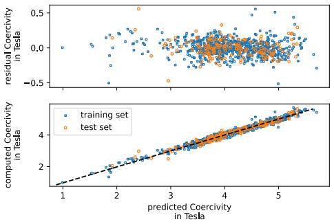
Pith's one-line read The paper claims that a single-layer graph neural network predicts the coercivity of Nd2Fe14B microstructures from grain geometry, orientation, and grain-boundary thickness with an $R^2$ of 96% on held-out simulations, and that the same…
desk verdict A solid in-distribution GNN surrogate for ROM-simulated coercivity, but the out-of-distribution claim needs a size-only baseline before it lands. read the letter →
The pith
A machine-rendered reading of the paper's core claim, the machinery that carries it, and where it could break.
The reading
What carries the argument
The load-bearing object is the graph encoding of a polycrystal: each grain becomes a node whose features are geometry, position, easy-axis orientation, and the field at which a single isolated grain would switch (the Stoner-Wohlfarth switching field), and each neighbouring grain pair becomes an edge whose feature is the non-magnetic grain-boundary thickness. The convolutional layer concatenates the source node, destination node, and edge features, applies a linear transformation with ReLU, and averages over one-hop neighbourhoods; this single message-passing hop is the mechanism that injects local demagnetizing-field physics without deep stacking. Above the convolution sit a global mean pooling and three fully connected layers that regress the scalar coercivity. The training labels come from a reduced-order micromagnetic model with a 2D surface mesh, analytic demagnetizing fields computed by surface integrals over polyhedra, and hierarchical-matrix acceleration. The out-of-distribution extension is carried by a logarithmic rescaling of edge-length-dependent features, justified by the fitted relation between coercivity and system size.
What would settle it
Train the same GNN on labels from full three-dimensional micromagnetic simulations (or from measured hysteresis loops of characterized NdFeB samples) for a matched set of microstructures, and compare predictions; if $R^2$ drops far below 96%, the reported accuracy is specific to the reduced-order model. Alternatively, simulate or measure physical magnets larger than 1.5 micrometers and check whether the $R^2 = 88$% out-of-distribution result persists beyond the size range used here.
Extended reading notes
Core claim
The paper's central claim is that a single message-passing layer, applied to a graph whose nodes are grains and whose edges are non-magnetic grain boundaries, captures enough local magnetostatic interaction to predict the coercive field of arbitrary grain mosaics. The model was trained on coercivity labels produced by a reduced-order micromagnetic simulator over a dataset spanning edge lengths from 179 nm to 68,326 nm and grain counts from 2 to 3,375, and it reproduces the simulator's coercivity on the held-out test set with $R^2 = 96$%. Beyond coercivity, the architecture is recycled for the maximum energy product, reaching $R^2 = 97$%, and for out-of-distribution structures larger than any seen in training it still achieves $R^2 = 88$% after log-scaling of size-dependent node features. The authors interpret the logarithmic feature scaling as encoding the observed size dependence of coercivity, which falls roughly as $H_c = -2.251 \cdot 10^{-2} \cdot \log_{1.05}(x/100) + 4.89$ with edge length $x$ in nm. If these results hold, a GNN trained once on simulator data can answer material-design questions about coercivity and energy product in fractions of the simulation time.
Load-bearing premise
The load-bearing premise is that the reduced-order simulator's computed coercivity is a faithful proxy for the coercivity of a real NdFeB magnet; if that proxy is biased, the GNN is only a fast emulator of the bias.
Editorial extensions
If this is right
- A single shallow GNN can replace the reduced-order simulator for coercivity screening: unseen microstructures are scored in a forward pass rather than by solving the magnetization-reversal problem.
- The same architecture transfers to a different target property (maximum energy product) with only added geometric features, suggesting a general encoder for polycrystalline magnets.
- Microstructures larger than 1.5 micrometers, which are the most expensive for micromagnetic simulation, can be predicted after log-scaling size-dependent features, with $R^2 = 88$%.
- The observed logarithmic fall of coercivity with system size is built into the model's feature scaling, making the model's extrapolation consistent with a known physical trend rather than a blind statistical extrapolation.
- For rare-earth-reduced magnet design, the model provides a fast objective function relating grain aspect ratio, sphericity, grain-boundary thickness, and easy-axis texture to coercivity and energy product.
Reading between the lines
- The reported $R^2$ values measure agreement with the reduced-order model, not with real magnets; the GNN's practical ceiling is therefore the ROM's fidelity to experiment, which the paper does not assess.
- The fact that one message-passing hop suffices suggests that, within the ROM, coercivity is dominated by local grain-neighbour interactions such as the cascade switching described in Section 7; deeper architectures may add little for this target.
- A natural testable extension is to train the same architecture on labels from full micromagnetic solvers or experimental hysteresis loops for a small matched set; the drop in $R^2$ would quantify how much of the ROM's bias the GNN inherits.
- The log-scaling trick, grounded in the fitted size law, could be reused for other size-dependent magnetic properties or for microstructures with different grain-boundary phases, and could be replaced by an explicit physical feature like the grain-size-dependent demagnetizing factor.
Editorial analysis
A structured set of objections, weighed in public.
Referee Report
Summary. The paper presents a graph neural network (GNN) surrogate trained on 1,054 microstructures simulated with a reduced-order micromagnetic model (ROM) to predict coercivity, achieving R²=96% on a held-out test set, and reuses the architecture to predict the maximum energy product with R²=97%. It also reports out-of-distribution generalization to microstructures larger than 1.5 µm, reaching R²=88% after log-scaling size-dependent features. The authors include uncertainty quantification via Monte-Carlo dropout and a Gaussian negative log-likelihood loss, and a confidence curve to validate the uncertainty estimates. The paper argues that the shallow single-convolutional-layer GNN with node and edge features captures the relevant microstructure physics.
Significance. If the reported results hold, the paper would be a useful demonstration of GNN surrogates for micromagnetic simulation, with potential to accelerate microstructure screening for permanent magnet design. The strengths include a reproducible open-source code and data release, a physically motivated feature set, explicit uncertainty quantification, and a clear application target (coercivity and energy product of Nd-Fe-B magnets). However, the central claim is conditional on the fidelity of the ROM and on the absence of trivial baselines; these gaps currently limit the significance for the broader materials community. The work is appropriately scoped as a surrogate-model study, and the feature-engineering insights tied to Section 7 provide a concrete physical rationale, but they also expose a potential circularity in the OOD claim.
major comments (3)
- [Sec. 6.3 and Sec. 7] The out-of-distribution generalization claim is not supported without a size-only baseline. The OOD test set differs from training primarily in edge length (all test structures >1.5 µm), and Section 7 independently shows that coercivity follows a near-logarithmic law Hc = -2.251e-2 * log1.05(x/100) + 4.89 for fixed parameters. Since the feature engineering in Sec. 6.3 explicitly applies log1.05 scaling to size-dependent features, the reported R²=88% may be trivially explained by this known size trend rather than by the GNN's message passing over grain features. Please report, on the same OOD split, the R² of (i) the Section 7 logarithmic fit using only edge length and (ii) a one-feature linear regression on log(edge length). If either baseline reaches ~88%, the claim of OOD generalization is not evidence of microstructure-aware learning.
- [Sec. 6.1 and Sec. 6.2] The reported R² values (96% and 97%) are point estimates without error bars, repeated-seed statistics, or baselines. Because the dataset size is modest (158 and ~170 test graphs) and the GNN has multiple hyperparameters, the performance could vary substantially across training runs. Please provide mean and standard deviation of R² over at least 5 independent restarts, and compare against simple baselines such as a linear regression on grain-averaged features, a multilayer perceptron with the same node features pooled, and a graph-mean predictor. This is essential to demonstrate that the GNN architecture, rather than the feature set or the size trend alone, drives the predictive accuracy.
- [Sec. 2 and Sec. 8] All training labels come from the reduced-order model, which assumes defect-free grains, non-magnetic grain boundaries, a 2D surface mesh, and analytic demagnetization fields. The paper never compares its predictions against experimental hysteresis loops, yet the title and abstract refer to predicting coercivity of hard magnetic microstructures without qualification. Please state this limitation prominently in the abstract or conclusions, and ideally include a small comparison with measured coercivity values from the literature for similar Nd-Fe-B microstructures. Without such a check, the practical significance of the GNN as a surrogate for real magnets remains unestablished; at minimum the claims should be framed as predictions of the ROM, not of physical coercivity.
minor comments (5)
- [Sec. 4.3] The text states that the learning rate is set to 9×10^-3, but Table 2 lists the optimized learning rate as 0.003. These numbers are inconsistent; please correct one of them.
- [Sec. 5, Eqs. (12)-(13)] In Eq. (12), the denominator inside the exponential is written as 2σ(x_i) but the normal distribution requires 2σ²(x_i); the same typo appears in the third term of Eq. (13). Please revise to make the variance appear as σ² throughout.
- [Sec. 5 and Sec. 6.1] It is not clear whether the results in Fig. 9 and the R²=96% are obtained with the model trained using the Huber loss (described in Sec. 4) or with the Gaussian negative log-likelihood loss (described in Sec. 5). If these are different models, please specify which one produced each result and how the hyperparameters differ.
- [Sec. 6.3 vs. Sec. 7] The feature-scaling formula in Sec. 6.3 is written as log1.05(1 + edge length/100), whereas the fitting function in Sec. 7 uses log1.05(x/100). Please clarify which form was actually used, because the additive constant affects the transformation materially for small x.
- [Fig. 4 caption] The caption labels both the global pooling layer and the final fully connected layer as '(d)', and the architecture list uses '(e)' for the three fully connected layers; please correct the label inconsistency.
Circularity Check
No significant circularity: the GNN's predictions are surrogate evaluations against a fixed ROM simulator, not derivations from its own outputs.
full rationale
The paper's central claims are surrogate-accuracy claims: a GNN is trained on labels generated by the authors' reduced-order model (Ref. [12]) and evaluated on held-out microstructures. This is a standard emulation setup, not a circular derivation, because the ROM's outputs are not functions of the GNN's predictions; the ROM is a published simulator with stated physical assumptions (defect-free grains, non-magnetic grain boundaries, 2D surface mesh, analytic demagnetization) and public code, so the citation [12] is genuine independent evidence for the label generator. The in-distribution R2=96% and BHmax R2=97% results are straightforward held-out evaluations. The OOD generalization experiment (Section 6.3) uses a log1.05 feature scaling that was motivated by the separately reported size-dependence analysis of Section 7, but the scaling is a feature transformation, not a fitted label predictor: the GNN still must learn the mapping to Hc from the scaled features, and the OOD test set contains varying aspect ratios and grain-boundary thicknesses, so the R2=88% is an empirical result rather than an identity. No equation in the paper reduces to another by construction, and no fitted parameter is renamed as a prediction. The ROM's fidelity to real experiments is a correctness risk, not a circularity, and the absence of a size-only baseline is a missing control rather than a circular step.
Assumptions & free parameters
free parameters (3)
- GNN hyperparameters (embedding size, learning rate, weight decay, dropout, batch size, epochs) =
18, 0.009, 0.0005, 0.6, 100, 150
- Log-size feature scaling base and offset =
log1.05(1 + edge_length/100)
- Size-dependence fit coefficients (Hc = -2.251e-2 * log1.05(x/100) + 4.89) =
-2.251e-2, 4.89
assumptions (3)
- domain assumption The reduced-order model accurately predicts coercivity and BHmax for hard magnetic microstructures
- domain assumption The graph representation of grains and grain boundaries captures the physical mechanisms that determine coercivity
- standard math Target errors are normally distributed and MC dropout estimates epistemic uncertainty
Cite this review
Pith. "Pith review of Graph Neural Networks to Predict Coercivity of Hard Magnetic Microstructures." pith.science (2026). https://pith.science/paper/3UXBSE5K
@misc{pith2026250623615,
  author       = {Pith},
  title        = {Pith review of: Graph Neural Networks to Predict Coercivity of Hard Magnetic Microstructures},
  year         = {2026},
  howpublished = {\url{https://pith.science/paper/3UXBSE5K}},
  note         = {Machine review of arXiv:2506.23615}
}
read the original abstract
Graph neural networks (GNN) are a promising tool to predict magnetic properties of large multi-grain structures, which can speed up the search for rare-earth free permanent magnets. In this paper, we use our magnetic simulation data to train a GNN to predict coercivity of hard magnetic microstructures. We evaluate the performance of the trained GNN and quantify its uncertainty. Subsequently, we reuse the GNN architecture for predicting the maximum energy product. Out-of-distribution predictions of coercivity are also performed, following feature engineering based on the observed dependence of coercivity on system size.
Figures


Figures from the paper (12 more)




Reference graph
Works this paper leans on
-
[1]
R. Skomski, J. Coey, Magnetic anisotropy — How much is enough for a permanent magnet?, Scripta Materialia 112 (2016) 3–8. doi:10.1016/ j.scriptamat.2015.09.021
work page 2016
-
[2]
N. Poudyal, J. Ping Liu, Advances in nanostructured permanent mag- nets research, Journal of Physics D: Applied Physics 46 (4) (2013) 043001. doi:10.1088/0022-3727/46/4/043001
-
[3]
A. Sanchez-Gonzalez, J. Godwin, T. Pfaff, R. Ying, J. Leskovec, P. Battaglia, Learning to simulate complex physics with graph networks, in: Proceedings of the 37th International Conference on Machine Learn- ing, Vol. 119, 2020, pp. 8459–8468
work page 2020
-
[4]
M. Dai, M. F. Demirel, X. Liu, Y. Liang, J.-M. Hu, Graph neural net- work for predicting the effective properties of polycrystalline materials: A comprehensive analysis, Computational Materials Science 230 (2023) 112461. doi:10.1016/j.commatsci.2023.112461. URL https://linkinghub.elsevier.com/retrieve/pii/ S092702562300455X
arXiv 2023
-
[5]
Y. Qin, S. DeWitt, B. Radhakrishnan, G. Biros, GrainNN: A neighbor-aware long short-term memory network for predict- ing microstructure evolution during polycrystalline grain for- mation, Computational Materials Science 218 (2023) 111927. doi:10.1016/j.commatsci.2022.111927. URL https://linkinghub.elsevier.com/retrieve/pii/ S0927025622006383
-
[6]
J. M. Hestroffer, M.-A. Charpagne, M. I. Latypov, I. J. Beyerlein, Graph neural networks for efficient learning of mechanical properties of polycrystals, Computational Materials Science 217 (2023) 111894. doi:10.1016/j.commatsci.2022.111894. URL https://linkinghub.elsevier.com/retrieve/pii/ S092702562200605X
arXiv 2023
-
[7]
W. Hamilton, Z. Ying, J. Leskovec, Inductive Representation Learning on Large Graphs, in: I. Guyon, U. V. Luxburg, S. Bengio, H. Wallach, 25 R. Fergus, S. Vishwanathan, R. Garnett (Eds.), Advances in Neural In- formation Processing Systems, Vol. 30, Curran Associates, Inc., 2017. URL https://proceedings.neurips.cc/paper_files/paper/2017/ file/5dd9db5e033d...
work page 2017
-
[8]
Paszke, S
A. Paszke, S. Gross, F. Massa, A. Lerer, J. Bradbury, G. Chanan, T. Killeen, Z. Lin, N. Gimelshein, L. Antiga, A. Desmaison, A. Kopf, E. Yang, Z. DeVito, M. Raison, A. Tejani, S. Chilamkurthy, B. Steiner, L. Fang, J. Bai, S. Chintala, Pytorch: An imperative style, high- performance deep learning library, in: Advances in Neural Information Processing Syste...
2019
Show all 39 references
- [9]
-
[10]
R. Quey, P. Dawson, F. Barbe, Large-scale 3D random polycrystals for the finite element method: Generation, meshing and remeshing, Com- puter Methods in Applied Mechanics and Engineering 200 (17-20) (2011) 1729–1745. doi:10.1016/j.cma.2011.01.002
2011 doi
-
[11]
Salom´ e, The Open Source Integration Platform for Numerical Simula- tion, www.salome-platform.org (Accessed: April 2025) (2025)
2025
-
[12]
Moustafa, A
H. Moustafa, A. Kovacs, J. Fischbacher, M. Gusenbauer, Q. Ali, L. Breth, Y. Hong, W. Rigaut, T. Devillers, N. M. Dempsey, T. Schrefl, H. Oezelt, Reduced order model for hard magnetic films, AIP Advances 14 (2) (2024) 025001. doi:10.1063/9.0000816. URL https://pubs.aip.org/adv/...
2024 doi
-
[13]
Singh, D
B. Singh, D. Guptasarma, New method for fast computation of gravity and magnetic anomalies from arbitrary polyhedra, GEOPHYSICS 66 (2) (2001) 521–526. doi:10.1190/1.1444942. URL https://library.seg.org/doi/10.1190/1.1444942
2001 doi
-
[14]
A. Y. Mikhalev, I. V. Oseledets, Iterative representing set selection for nested cross approximation, Numerical Linear Algebra with Applica- tions 23 (2) (2016) 230–248. doi:10.1002/nla.2021. URL https://onlinelibrary.wiley.com/doi/10.1002/nla.2021 26
2016 doi
-
[15]
Marsaglia, Choosing a Point from the Surface of a Sphere, The Annals of Mathematical Statistics 43 (2) (1972) 645–646
G. Marsaglia, Choosing a Point from the Surface of a Sphere, The Annals of Mathematical Statistics 43 (2) (1972) 645–646. doi:10.1214/aoms/ 1177692644. URL http://projecteuclid.org/euclid.aoms/1177692644
1972
-
[16]
A. G´ eron, Hands-on machine learning with Scikit-Learn, Keras, and TensorFlow: concepts, tools, and techniques to build intelligent sys- tems, second edition Edition, O’Reilly Media, Inc, Beijing [China] ; Se- bastopol, CA, 2019
2019
-
[17]
Pedregosa, G
F. Pedregosa, G. Varoquaux, A. Gramfort, V. Michel, B. Thirion, O. Grisel, M. Blondel, P. Prettenhofer, R. Weiss, V. Dubourg, J. Vander- plas, A. Passos, D. Cournapeau, M. Brucher, M. Perrot, E. Duchesnay, Scikit-learn: Machine learning in Python, Journal of Machine Learning R...
2011
-
[18]
Permutation feature importance
4.2. Permutation feature importance. URL https://scikit-learn.org/stable/modules/permutation_ importance.html
- [19]
-
[20]
S. Park, N. Kwak, Analysis on the Dropout Effect in Convolutional Neural Networks, in: S.-H. Lai, V. Lepetit, K. Nishino, Y. Sato (Eds.), Computer Vision – ACCV 2016, Vol. 10112, Springer International Pub- lishing, Cham, 2017, pp. 189–204, series Title: Lecture Notes in Com- ...
2016 doi
- [21]
- [22]
-
[23]
P. Zhou, X. Xie, Z. Lin, S. Yan, Towards Understanding Convergence and Generalization of AdamW, IEEE Transactions on Pattern Analysis and Machine Intelligence 46 (9) (2024) 6486–6493.doi:10.1109/TPAMI. 2024.3382294. URL https://ieeexplore.ieee.org/document/10480574/
2024
-
[24]
P. J. Huber, Robust Estimation of a Location Parameter, The Annals of Mathematical Statistics 35 (1) (1964) 73–101. doi:10.1214/aoms/ 1177703732. URL http://projecteuclid.org/euclid.aoms/1177703732
1964
- [25]
-
[26]
Y. Hu, A. Levi, I. Kumar, Y. Zhang, M. Coates, On batch size selection for stochastic training for graph neural networks, ICLR 2021 Conference (Sep. 2020)
2021
-
[27]
Broadwater, Graph Neural Networks in Action, Manning Publica- tions, US, 2025, oCLC: 1482783825
K. Broadwater, Graph Neural Networks in Action, Manning Publica- tions, US, 2025, oCLC: 1482783825
2025
- [28]
-
[29]
Gawlikowski, C
J. Gawlikowski, C. R. N. Tassi, M. Ali, J. Lee, M. Humt, J. Feng, A. Kruspe, R. Triebel, P. Jung, R. Roscher, M. Shahzad, W. Yang, R. Bamler, X. X. Zhu, A survey of uncertainty in deep neural networks, Artificial Intelligence Review 56 (S1) (2023) 1513–1589. doi:10.1007/ s1046...
2023 doi
-
[30]
D. Nix, A. Weigend, Estimating the mean and variance of the target probability distribution, in: Proceedings of 1994 IEEE International Conference on Neural Networks (ICNN’94), IEEE, Orlando, FL, USA, 28 1994, pp. 55–60 vol.1. doi:10.1109/ICNN.1994.374138. URL http://ieeexplor...
1994
- [31]
-
[32]
A. D. Kiureghian, O. Ditlevsen, Aleatory or epistemic? Does it matter?, Structural Safety 31 (2) (2009) 105–112. doi:10.1016/j.strusafe.2008.06.020. URL https://linkinghub.elsevier.com/retrieve/pii/ S0167473008000556
2009 doi
-
[33]
S. Ryu, Y. Kwon, W. Y. Kim, A Bayesian graph convolutional network for reliable prediction of molecular properties with uncertainty quan- tification, Chemical Science 10 (36) (2019) 8438–8446. doi:10.1039/ C9SC01992H. URL https://xlink.rsc.org/?DOI=C9SC01992H
2019
- [34]
-
[35]
Project, Magnetic materials ontology, https://github.com/ MaMMoS-project/MagneticMaterialsOntology, accessed: 2025-05-21 (2024)
M. Project, Magnetic materials ontology, https://github.com/ MaMMoS-project/MagneticMaterialsOntology, accessed: 2025-05-21 (2024)
2024
-
[36]
S. Fan, X. Wang, C. Shi, P. Cui, B. Wang, Generalizing Graph Neural Networks on Out-of-Distribution Graphs, IEEE Transactions on Pattern Analysis and Machine Intelligence 46 (1) (2024) 322–337. doi:10.1109/ TPAMI.2023.3321097. URL https://ieeexplore.ieee.org/document/10268633/
2024
- [37]
-
[38]
Bance, B
S. Bance, B. Seebacher, T. Schrefl, L. Exl, M. Winklhofer, G. Hrkac, G. Zimanyi, T. Shoji, M. Yano, N. Sakuma, M. Ito, A. Kato, A. Man- abe, Grain-size dependent demagnetizing factors in permanent magnets, Journal of Applied Physics 116 (23) (2014) 233903. doi:10.1063/1. 49048...
2014 doi
-
[39]
Kovacs, J
A. Kovacs, J. Fischbacher, H. Oezelt, A. Kornell, Q. Ali, M. Gusen- bauer, M. Yano, N. Sakuma, A. Kinoshita, T. Shoji, A. Kato, Y. Hong, S. Grenier, T. Devillers, N. M. Dempsey, T. Fukushima, H. Akai, N. Kawashima, T. Miyake, T. Schrefl, Physics-informed machine learn- ing com...
2023 doi
Reviewed August 6, 2026 · model on record in the stance chip above.
Discussion (0). Continue with ORCID to comment.