REVIEW 4 major objections 6 minor 10 references
Position-Normal Manifold for Efficient Glint Rendering on High-Resolution Normal Maps
T0 review · 4 major / 6 minor · reviewed 2026-08-15 · deepseek-v4-flash
Pith's one-line read Exact glint NDF evaluation via 4D manifold intersections
desk verdict Genuinely new closed-form P-NDF evaluation and analytical shadow-masking, but the 'exact' label overstates what the renderer actually uses; worth a serious referee with a request for sensitivity analysis. read the letter →
The pith
A machine-rendered reading of the paper's core claim, the machinery that carries it, and where it could break.
The reading
What carries the argument
The load-bearing object is the position-normal manifold: the graph $(u, n(u))$ of the normal map, triangulated into a 4D mesh with barycentric normal interpolation. Evaluating the P-NDF is then projection of this manifold onto the normal plane, implemented as point-in-triangle tests between the query normal $m$ and normal triangles $n(\triangle abc)$, followed by accumulating kernel-weighted inverse-Jacobian contributions. A min-max bounding hierarchy prunes triangles that cannot intersect the query, and a cluster hierarchy approximates large footprints with coarser grids whose normals are fit by weighted least squares. For shadow-masking, Stokes' theorem converts the projected-area integral over each clipped normal triangle into closed-form line integrals over straight edges and ellipse arcs.
What would settle it
Render a specular surface with several normal maps containing large flat regions and isolated tiny bumps, and compare images at epsilon = $10^{-8}$, $10^{-6}$, and $10^{-4}$ at the same sample count; if maximum highlight intensity or glint density changes by more than a few percent, the clamped-pdf claim collapses. A direct check is to compute the true Gaussian-convolved NDF by brute-force binning for such maps and measure the error of the clamped-pdf P-NDF against it.
Extended reading notes
Core claim
At its center is the claim that Eq. (5) of the paper is an exact solution of Eq. (2) for a piecewise-linear normal map: $$D(m,x) = \sum_{\triangle abc \in k_r} \frac{k_r(a\lambda_0+b\lambda_1+c\lambda_2 - x)\,\mathbf{1}_{n(\triangle abc)}(m)}{2\|n(\triangle abc)\|}.$$ Each normal triangle $n(\triangle abc)$ that contains the queried normal $m$ contributes, and the kernel weight is evaluated at the barycentric texture coordinate of the intersection, normalized by twice the triangle's area in normal space. Because this is a direct evaluation of the un-convolved footprint NDF, the Gaussian micro-roughness convolution required by earlier continuous glint models is avoided; degenerate zero-area triangles are instead handled by clamping the Jacobian to $\epsilon = 10^{-6}$. The same manifold view extends to shadowing-masking: with a piecewise-constant footprint kernel, the projected-area integral over each normal triangle becomes the area of the triangle clipped against a semi-circle and semi-ellipse, and Stokes' theorem converts that area into closed-form line integrals. In short, the paper establishes an exact, mesh-intersection formulation of glint NDFs together with an analytical shadow-masking term.
Load-bearing premise
The load-bearing premise is that replacing triangles whose Jacobian is below epsilon = $10^{-6}$ with a clamped equilateral triangle of exactly that area reproduces the appearance of Gaussian-convolved glints; the paper does not test how sensitive the rendered highlights are to the clamp size or shape.
Editorial extensions
If this is right
- At footprint scales near 256 by 256 texels, the full hierarchy brings render time from tens of minutes to about a minute on the test scenes, so the same time budget can buy many more samples per pixel.
- Because evaluation no longer requires Gaussian kernel convolutions, arbitrary footprint kernels such as disk or box filters can be substituted; on the isotropic test map, a disk or box filter at half footprint reaches similar NDFs at roughly twice the speed.
- The analytical projected-area integral supplies a shadow-masking term for the continuous glint BRDF that prior continuous formulations lacked, improving grazing-angle behavior.
- For diffuse surfaces, aggregating the projected area inside the pixel footprint removes aliasing from normal-mapped diffuse reflections at 1 sample per pixel while preserving microstructure detail.
Reading between the lines
- A testable extension is to treat the clamp epsilon as a user-facing glint sharpness parameter: the same mesh machinery could quantify how glint peak height and sparkle density scale with epsilon, a sensitivity study the paper does not run.
- The point-in-triangle formulation maps directly onto ray-tracing hardware; building the normal-triangle mesh as a bounding-volume hierarchy and querying it with a ray along the desired normal could plausibly push glint evaluation to interactive rates.
- The analytical projected area could be reused as a building block for multiple-scattering or interreflection corrections on the microsurface, which the paper identifies as an open direction.
Signed reviews
Editorial analysis
A structured set of objections, weighed in public.
Referee Report
Summary. The paper presents a manifold-based formulation for glint rendering on high-resolution normal maps. The authors represent the graph of a continuous normal map as a 4D position-normal triangle mesh and show that P-NDF evaluation reduces to point-triangle intersections, giving Eq. (5) as a closed-form sum that is exact for the piecewise-linear representation. They add a min-max hierarchy and a mesh-clustering hierarchy to accelerate large-footprint queries, and they replace near-singular Jacobian determinants by a clamped value epsilon. The same framework is extended to an analytical projected-area/shadow-masking integral, Eq. (12), with a GGX approximation, and this is applied to anti-aliased normal-mapped diffuse rendering. The results report quality similar to Yan et al. [2014, 2016] with large speedups, especially for large footprint sizes.
Significance. If the claims hold, this is a significant contribution to glint rendering: the P-NDF identity in Eq. (5) is an elegant, parameter-free solution of the continuous formulation, and the reported speedups of roughly one order of magnitude over Yan et al. [2016] are practically important. The analytical projected-area derivation for shadow-masking and diffuse anti-aliasing is a novel extension that fills a gap in prior continuous glint models. The paper is also commendable for releasing code, validating Eq. (5) against binning and Monte Carlo references, and supplying detailed appendix derivations. The main reservations are that the exact identity is not what the renderer actually evaluates, and the two approximations used in practice -- Jacobian clamping and cluster-based approximation -- are validated only qualitatively or against the authors' own no-cluster baseline.
major comments (4)
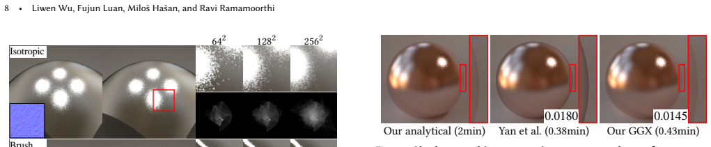
- [Sec. 4.1, Eqs. (5)-(6), Fig. 4] The central exactness claim applies to the unclamped singular P-NDF in Eq. (5), but the actual renderer samples and evaluates the clamped pdf of Eq. (6). The sentence 'an alternative strategy by clamping is just as effective' is not supported by quantitative evidence: no sensitivity analysis on epsilon is reported, no error metric against the Gaussian-convolved reference is given, and Fig. 4 is a single qualitative comparison on one normal map. Since clamping directly sets the height of glint peaks exactly where the Jacobian singularities live, a factor of 10 in epsilon changes peak densities by an order of magnitude. Moreover, epsilon is an absolute threshold while normal-map Jacobians carry units of normal area per texel area, so the same epsilon cannot be expected to behave identically across texture resolutions and footprint scales. The authors should provide an epsilon sensitivity study, compare the clamped pdf against the convolved reference quantitatively, and either justify the absolute threshold or propose a relative or size-aware clamping rule.
- [Sec. 4.2, Eqs. (7)-(8), Fig. 15, Tab. 3] The cluster hierarchy changes the P-NDF itself: sampling uses n^l(u/2^l) rather than the original normal map, so the evaluated density is no longer the exact Eq. (5) density. The residual threshold tau is a heuristic chosen per scene (10^-3 in general but 10^-4 for the scratch map in Sec. 5.1), and no error bound connecting the least-squares residual to P-NDF error is given. The ablation in Tab. 3 and Fig. 15 compares clustered against the non-clustered version of the same method, not against the exact Eq. (2) or against the convolved reference, so the claim that the glint pattern is 'well-preserved' is not quantitatively established. I ask the authors to report P-NDF error or rendering error with respect to the unclustered exact evaluation for several tau values and several maps, and to state the tau selection rule independently of the scene.
- [Sec. 4.3, Eqs. (9)-(10)] Eq. (9) writes P(omega) as an integral over d\tilde m, while Eq. (10) introduces a 1/\tilde m_z factor when passing to the projected-coordinate measure dm. As written, the two equations are inconsistent in their integration measure: if d\tilde m denotes projected area, the notation should be dm; if d\tilde m denotes solid angle, then a Jacobian factor belongs in Eq. (9). Since the analytical shadow-masking contribution rests on this projected-area derivation, the measure convention must be stated explicitly and used consistently from Eq. (9) onward.
- [Sec. 5.1, Tab. 2, Sec. 5.3, Tab. 3] The reported speedups are partly parameter-dependent: the clustering threshold tau is set to 10^-3 for isotropic and brush maps but 10^-4 for the scratch map, and the disk/box-filter experiments in Sec. 5.3 use different footprint sizes than the Gaussian experiments. This makes the headline 'order of magnitude faster' difficult to interpret as a property of the method rather than of the chosen operating points. Please report timing and error for a common parameter configuration, and show how the speedup varies with tau over at least a small grid, so readers can assess the robustness of the comparison.
minor comments (6)
- [Fig. 4] The caption 'Binning With convolution' is unclear; please specify which panel is the binning reference, which is the convolved reference, and what the shown error values measure.
- [Sec. 4.1, Eq. (3)] The vertex labels n0...n3 are used before their correspondence to u0...u3 is stated; consider adding an explicit equation or sentence defining n_i = n(u_i) immediately before Eq. (3).
- [Abstract and Sec. 4.1] The word 'exact' in the abstract conflicts with the clamping step in Eq. (6); suggest hedging the abstract to 'exact for the piecewise-linear normal map up to the singularity treatment'.
- [Sec. 5.2] The statement that Yan et al. [2014, 2016] 'simply take the Beckmann shadow-masking using fixed roughness' should specify the roughness value used, otherwise the comparison is not reproducible.
- [Sec. 5.3, Fig. 16] The disk/box-filter comparison uses a different footprint scale than the Gaussian case; please state the effective kernel widths explicitly in the text or caption so the comparison is interpretable.
- [Appendix A, Eq. (15)] The cluster-domain notation with translated coordinates is difficult to follow; a short worked example for l=1 would help readers verify the least-squares setup.
Circularity Check
No significant circularity: the core manifold-intersection derivation is self-contained; the clamp and GGX approximations are labeled approximations, not predictions.
full rationale
The central derivation, Eq. (5), is obtained directly from the defining delta-integral in Eq. (2) by representing the normal map as a piecewise-linear mesh and summing the kernel-weighted Jacobian contributions over each intersecting normal triangle. This is a change of variables over the same quantity being defined, not a separate fitted input, so the claim that Eq. (5) is an exact solution of Eq. (2) is self-contained. The clamping operation in Sec. 4.1, Eq. (6), replaces near-singular triangles with small equilateral triangles; this is an explicit regularization of the clamped PDF, and the paper states that the clamping is 'just as effective' as Yan et al.'s Gaussian convolution. That assertion is a validation gap or correctness risk, but it is not circular: the clamped PDF is defined independently and compared against the convolved reference in Fig. 4, and no hidden parameter is reused as the target result. The cluster hierarchy in Sec. 4.2 fits cluster normals by weighted least squares (Eqs. 7-8) to approximate the original normal map; this is a clearly labeled approximation with an ablation in Fig. 15 and Tab. 3, not a prediction of the exact P-NDF. The shadow-masking derivation in Sec. 4.3 follows from an exact projected-area integral via Stokes' theorem, and the GGX fit in Eq. (13) is explicitly said to be an approximation fitted to the paper's own analytical projected-area function. Self-citations to Yan et al. [2014, 2016] are used as baselines and as prior formulation context; the correctness of Eq. (5), Eq. (12), and the diffuse BRDF aggregation in Eq. (14) does not depend on those papers' theorems or fitted values. No self-referential theorem is invoked to forbid alternatives, and no known result is renamed as a new derivation. Therefore the paper shows no circularity in its central claim.
Assumptions & free parameters
free parameters (3)
- epsilon =
1e-6
- tau =
1e-3 to 1e-4
- GGX roughness alpha and tangent frame Q =
fitted via least squares
assumptions (5)
- domain assumption The normal map is piecewise-linear over each texel's two triangles (barycentric interpolation).
- domain assumption The microfacet BRDF follows the Smith shadowing-masking model with Lambda(omega) = P(omega)/omega_z - 1.
- domain assumption The footprint kernel k_r is treated as piecewise constant per triangle for the analytical projected-area integral.
- domain assumption Diffuse microfacets are Lambertian with the projection factor 1/n_z used for the surface area measure.
- ad hoc to paper Clamping the Jacobian at epsilon yields a P-NDF visually equivalent to the Gaussian-convolved P-NDF.
Cite this review
Pith. "Pith review of Position-Normal Manifold for Efficient Glint Rendering on High-Resolution Normal Maps." pith.science (2026). https://pith.science/paper/3XW7QH6T
@misc{pith2026250508985,
  author       = {Pith},
  title        = {Pith review of: Position-Normal Manifold for Efficient Glint Rendering on High-Resolution Normal Maps},
  year         = {2026},
  howpublished = {\url{https://pith.science/paper/3XW7QH6T}},
  note         = {Machine review of arXiv:2505.08985}
}
read the original abstract
Detailed microstructures on specular objects often exhibit intriguing glinty patterns under high-frequency lighting, which is challenging to render using a conventional normal-mapped BRDF. In this paper, we present a manifold-based formulation of the glint normal distribution functions (NDF) that precisely captures the surface normal distributions over queried footprints. The manifold-based formulation transfers the integration for the glint NDF construction to a problem of mesh intersections. Compared to previous works that rely on complex numerical approximations, our integral solution is exact and much simpler to compute, which also allows an easy adaptation of a mesh clustering hierarchy to accelerate the NDF evaluation of large footprints. Our performance and quality analysis shows that our NDF formulation achieves similar glinty appearance compared to the baselines but is an order of magnitude faster. Within this framework, we further present a novel derivation of analytical shadow-masking for normal-mapped diffuse surfaces -- a component that is often ignored in previous works.
Figures


Figures from the paper (16 more)




Reference graph
Works this paper leans on
-
[2016]
that use intrinsic roughness, Additional comparison with Yan et al. [2016]. Figure 19 shows qual- itative comparison with Yan et al. under different footprint scales on scenes in Fig. 9 of the paper. We additionally show renderings using the flake normal map with coating, whose timing is provided in Tab
work page 2016
-
[5]
journal of graphics tools 10, 3 (2005), 65–71
Mipmapping normal maps. journal of graphics tools 10, 3 (2005), 65–71. Bruce Walter, Sebastian Fernandez, Adam Arbree, Kavita Bala, Michael Donikian, and Donald P Greenberg
work page 2005
-
[10]
and our evaluation without the clustering (ours no cluster) demonstrate faster inference speed compared to their performances on other normal maps. Timing of different stages. Table 5 shows the timing of different rendering stages for the scenes in Fig. 14 of the paper. For indirect bounces, Mitsuba [Jakob 2010] sets their ray differentials to zero that c...
work page 2010
-
[14]
(26) C Experiment details Entry level of the acceleration structures
Direct BRDF Direct emitter Indirect Total Wrench 0.31 0.14 0.19 0.63 Kettle 0.21 0.12 0.15 0.48 Plate & Cutlery 0.72 0.22 0.10 1.04 The cosine term between the line and the ˜m𝑦 axis is d𝑥 , thus, the line integral of 𝝎𝑥 ˜m𝑧 is: ∮ n𝑖+1 n𝑖 𝝎𝑥 ˜m𝑧d ˜m𝑦 = 𝝎𝑥 2 𝑟 2d𝑦 h arcsin𝑝+𝑝 √︁ 1−𝑝2 i d⊤n𝑖+1/𝑟 d⊤n𝑖/𝑟 . (26) C Experiment details Entry level of the accelerat...
work page 1994
-
[1967]
Haowen Tan, Junqiu Zhu, Yanning Xu, Xiangxu Meng, Lu Wang, and Ling-Qi Yan
Geometrical shadowing of a random rough surface.IEEE transactions on antennas and propagation 15, 5 (1967), 668–671. Haowen Tan, Junqiu Zhu, Yanning Xu, Xiangxu Meng, Lu Wang, and Ling-Qi Yan
work page 1967
-
[2005]
JOSA A 22, 11 (2005), 2442–2453
Detailed analytical approach to the Gaussian surface bidirectional reflectance distribution function specular component applied to the sea surface. JOSA A 22, 11 (2005), 2442–2453. Ishaan Shah, Luis E Gamboa, Adrien Gruson, and PJ Narayanan
work page 2005
-
[2007]
Microfacet models for refraction through rough surfaces. In EGSR. Beibei Wang, Miloš Hašan, Nicolas Holzschuch, and Ling-Qi Yan. 2020b. Example-based microstructure rendering with constant storage. Beibei Wang, Miloš Hašan, and Ling-Qi Yan. 2020a. Path cuts: Efficient rendering of pure specular light transport. ACM TOG (2020). Beibei Wang, Lu Wang, and Ni...
work page 2020
-
[2021]
InSIGGRAPH 2021 Course: Advances in Real-Time Rendering in Games
Nanite a deep dive. InSIGGRAPH 2021 Course: Advances in Real-Time Rendering in Games . Alexandr Kuznetsov
work page 2021
Show all 10 references
-
[2022]
IEEE Trans- actions on Visualization and Computer Graphics (2022)
Efficient Specular Glints Rendering With Differentiable Regularization. IEEE Trans- actions on Visualization and Computer Graphics (2022). Zhimin Fan, Jie Guo, Yiming Wang, Tianyu Xiao, Hao Zhang, Chenxi Zhou, Zhenyu Chen, Pengpei Hong, Yanwen Guo, and Ling-Qi Yan
2022
-
[2023]
arXiv preprint arXiv:2305.02678 (2023)
Real-time neural appearance models. arXiv preprint arXiv:2305.02678 (2023). Shuang Zhao, Lifan Wu, Frédo Durand, and Ravi Ramamoorthi
2023 arXiv
Reviewed August 15, 2026 · model on record in the stance chip above.
Discussion (0). Continue with ORCID to comment.