REVIEW 1 major objections 5 minor 42 references
Nonparametric Inference for Noise Covariance Kernels in Parabolic SPDEs using Space-Time Infill-Asymptotics
T0 review · 1 major / 5 minor · reviewed 2026-08-05 · deepseek-v4-flash
Pith's one-line read A discretized infinite-dimensional realized covariation estimates the full noise covariance of a linear parabolic SPDE without knowing the elliptic operator, and its CLT supports omnibus goodness-of-fit tests.
desk verdict Solid extension of realized covariation to discrete sampling and unknown A, with one real but fixable gap in the local-average CLT. read the letter →
The pith
A machine-rendered reading of the paper's core claim, the machinery that carries it, and where it could break.
The reading
What carries the argument
The central object is the infinite-dimensional realized covariation RV_T^{Δ,O} = Σ_i (OX_{iΔ} − OX_{(i−1)Δ})^{⊗2}, normalized by T, where ⊗ denotes the Hilbert-space tensor square and O is the spatial observation operator: I for continuous data, the L^2 projection P_h for local averages, and the piecewise-linear interpolant I_h for pointwise data. The estimator is compared with a semigroup-adjusted version SARCV_T^{Δ,O} = Σ_i (OX_{iΔ} − OS(Δ)X_{(i−1)Δ})^{⊗2}; the difference is shown to be negligible, so the limit theory of the latter transfers. The analytic semigroup S(t) = e^{−tA} supplies the smoothing estimates that force the bias term involving the initial value to vanish. The limiting c
What would settle it
Take the same SPDE but replace A by a non-analytic semigroup generator, such as a hyperbolic wave-type operator with imaginary spectrum, keep the same trace-class Q and X0 = 0, and compute the Hilbert–Schmidt distance between RV_T^{Δ,O}/T and Q as Δ, h → 0; if it does not converge to 0, the identifiability claim fails outside the analytic class. Within the assumptions, a Monte-Carlo check of the CLT for A = −Δ_D, Q = (−Δ_D)^{−σ}, O = I_h with h = O(Δ^{3/8}) in d = 3, comparing the empirical covariance of Δ^{−1/2}(RV/T − Q) against Γ = Q(· + ·*)Q, would falsify the normality claim if the match
Extended reading notes
Core claim
Formally, the paper proves that under Assumption 1, RV_T^{Δ,I}/T converges to Q in L^2(Ω, L2(H)) as Δ↓0, giving identifiability of the whole kernel. Under Assumption 2 with 2ι ≥ γ ≥ 1, for each of the three observation schemes—identity (continuous spatial data), orthogonal projection onto piecewise constants (local averages), and piecewise linear interpolation (pointwise data)—one has Δ^{-1/2}(RV_T^{Δ,O}/T − Q) converging in distribution to N(0, Γ) in the Hilbert–Schmidt norm, with ΓB = Q(B + B*)Q. The discrete spatial schemes require coupling the mesh size h to the time step Δ: h = o(Δ^{1/2}) for local averages, and h = O(Δ^{3/(2d+2)}) for d ≤ 2 or O(Δ^{3/8}) for d = 3 for pointwise samplin
Load-bearing premise
The load-bearing premise is that the differential operator A is self-adjoint, positive definite with compact inverse, so that its semigroup is analytic and smooths the initial state exponentially; without that smoothing, the realized covariation need not converge to Q.
Editorial extensions
If this is right
- For any linear parabolic SPDE satisfying the assumptions, the full noise covariance kernel can be estimated consistently from space-time data, so noise-model validation can be separated from estimation of the differential operator.
- The CLT gives asymptotic normality at rate √Δ when the smoothness exponent γ ≥ 1, matching the canonical finite-dimensional semimartingale rate, and spatial resolution may be coarser than temporal resolution.
- An omnibus goodness-of-fit test for a fixed hypothesized kernel Q0 is asymptotically of exact level α, with a computable generalized-χ² null distribution.
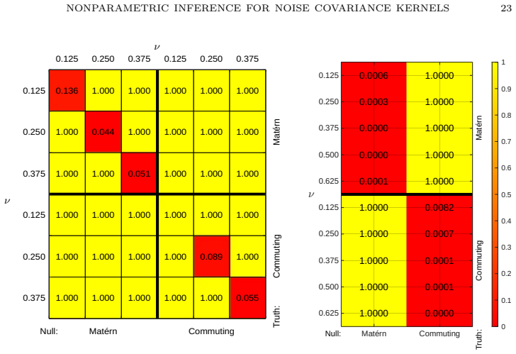
- A conservative test for parametric families such as Matérn or inverse-fractional-Laplacian covariances is asymptotically of level at most α and exhibits high power against qualitatively different kernel families.
- When the regularity conditions fail, such as low Matérn smoothness, the empirical size of the test drifts away from α, confirming the conditions are needed and not merely technical.
Reading between the lines
- Editorial inference: Because Γ is built from Q alone, the same CLT yields asymptotic confidence ellipsoids for the kernel by plugging the estimated Q into Γ; the paper constructs tests, but the covariance formula is ready-made for interval construction.
- Editorial inference: The proof's reliance on polynomial-approximation bounds suggests the estimator extends to other observation schemes, such as weighted averages, finite-element projections, or irregular grids, with rates set by ∥O−I∥ and the same CLT whenever the semigroup remains analytic.
- Editorial inference: The paper notes the bias does not vanish as T→∞ for fixed Δ; a natural next step, implicit in Remark 4.8, is to estimate and subtract the bias using long time spans, which would extend the √Δ CLT to settings where bias currently dominates.
Editorial analysis
A structured set of objections, weighed in public.
Referee Report
Summary. The paper develops asymptotic inference for the trace-class spatial covariance operator Q of the additive noise in a linear parabolic SPDE, based on realized covariations of the solution under space-time infill asymptotics. The central results are: (i) consistency of RV_T^{Δ,O}/T for Q in Hilbert-Schmidt norm under a general self-adjoint elliptic operator A, with A unknown; (ii) convergence rates for three sampling schemes (continuous observation, local averages, pointwise interpolation) depending on regularity parameters; (iii) a CLT of the form Δ^{-1/2}(RV_T^{Δ,O}/T - Q) ⇒ N(0,Γ) with ΓB = Q(B+B*)Q under Assumption 2 with 2ι ≥ γ ≥ 1; and (iv) omnibus goodness-of-fit tests for fixed and parametric covariance hypotheses. The proofs are detailed in an appendix, and a simulation study examines rates, size, and power.
Significance. If the stated results hold, this is a substantial contribution to statistical inference for parabolic SPDEs. The main novelty—estimating the full noise covariance operator nonparametrically from realized covariations without knowing A—is of real practical value, and the paper backs it with explicit rates, a CLT whose covariance depends only on Q, a lower bound showing near-optimality, and a careful treatment of three sampling designs. The simulation study is honest, explicitly showing size distortion when the regularity conditions of the CLT fail. The proofs are detailed and the assumptions are illustrated with natural examples (Matérn kernels, fractional inverse Laplacians). These strengths make the manuscript worth publishing after revision.
major comments (1)
- [Theorem 4.13(B) and Lemma B.9] The proof of part (B) of Theorem 4.13 relies on Lemma B.9 to show that the local-average semigroup-adjusted covariation is asymptotically equivalent to the identity-observation version (term IV in the proof of Theorem 4.13). Lemma B.9, however, is proved only for nested subdivisions (T_h): the proof uses monotone convergence of ∥(I−P_h)v∥ and Dini's theorem to obtain sup_{r≤1}∥(P_h−I)S(r)Q^{1/2}∥_{L2(H)}→0. Theorem 4.13(B) and Section 3(B) only assume a non-degenerate family of subdivisions and h=o(Δ^{1/2}); no nestedness is stated. Without nestedness (or a different direct compactness argument), the uniform convergence is not established, and the displayed o_p(T^{1/2}Δ^{1/2}) bound for the difference between the P_h and I realized covariations does not follow. Since part (B) is one of the three sampling schemes in the paper's central CLT, this is a load-bearing gap. It is fixable by add
minor comments (5)
- [Lemma B.9, second bullet] The displayed condition for O=I_h, 'h = o(Δ^{(tilde-epsilon-1)/(2 min(psi,2))})', does not match the condition used in Theorem 4.13(C), and appears to contain a typo in the exponent. Please check and harmonize the statement with the proof and with Theorem 4.13(C).
- [Theorem 5.4 proof] In the proof, the line 'T(θ0)=0 < T(θ0)' should read '0 < T(θ)' for θ ≠ θ0.
- [Theorem 4.9(C)] There is a typo: 'Assumption 4 is satisfied and and that' should be 'and that'.
- [Algorithm 2] The instruction 'Proceed with Steps 3–4 of Algorithm 1' is ambiguous because the test statistic has already been computed in Algorithm 2; it should say 'Proceed with Steps 4–6 of Algorithm 1' or equivalent.
- [Section 3(B) and Section 4.3] If the nested condition is indeed required for Theorem 4.13(B), it should be introduced in Section 3(B) as part of the definition of the sampling scheme, not only inside a lemma in the appendix.
Circularity Check
No significant circularity: the paper's claims reduce to an independently established semigroup-adjusted CLT, not to their own definitions or fitted inputs.
full rationale
The estimation target Q is the trace-class covariance of the driving Wiener process, defined independently of the estimator RV_T^{Δ,O}/T. The central CLT (Theorem 4.13) is proved by decomposing the discretely sampled realized covariation into remainders (Lemmas B.1, B.2, B.4, B.6, B.7, B.9) plus the semigroup-adjusted estimator SARCV^{Δ,I}, whose asymptotic normality is quoted from the prior work [5, 6, 7] (Theorem D.10 in [7]). Although one present author (Schroers) is a coauthor of those prior papers, the cited results are published mathematical theorems with their own proofs and do not themselves assume the conclusion of this paper; they are not fitted to any data, and they do not define Q in terms of the statistic. The new sampling schemes (B) and (C) are handled by showing that the projection/interpolation error is asymptotically negligible, which is genuine new content. The proof of Theorem 4.13(B) as written uses a nested-subdivision condition in Lemma B.9 that is not stated in the theorem; this is a potential correctness gap in the proof, but it is not circularity, because the missing condition is a hypothesis on the mesh, not the target Q. No parameter is fitted and then renamed a prediction, and no known empirical pattern is repackaged as a derivation. Accordingly the circularity score is 0.
Assumptions & free parameters
assumptions (7)
- domain assumption A is closed, densely defined, self-adjoint, positive definite on H with compact inverse (Assumption 1)
- domain assumption Q is trace-class and X0 ∈ L4(Ω,H) (Assumption 1)
- domain assumption Regularity conditions of Assumption 2: ∥A^{γ/2}Q∥_{L2}<∞ and ∥A^{ι/2}X0∥_{L4}<∞
- domain assumption Assumption 3: ˙H^1 ↪ H^1 (for local averages)
- domain assumption Assumption 4: stronger operator-norm regularity and ˙H^2 ↪ H^2 (for pointwise sampling)
- ad hoc to paper Nested subdivisions of T_h in Lemma B.9 for O=Ph
- standard math Standard Itô isometry, BDG inequality, spectral calculus, embedding theorems
Cite this review
Pith. "Pith review of Nonparametric Inference for Noise Covariance Kernels in Parabolic SPDEs using Space-Time Infill-Asymptotics." pith.science (2026). https://pith.science/paper/43IZFHIY
@misc{pith2026250820947,
  author       = {Pith},
  title        = {Pith review of: Nonparametric Inference for Noise Covariance Kernels in Parabolic SPDEs using Space-Time Infill-Asymptotics},
  year         = {2026},
  howpublished = {\url{https://pith.science/paper/43IZFHIY}},
  note         = {Machine review of arXiv:2508.20947}
}
read the original abstract
We develop an asymptotic limit theory for nonparametric estimation of the noise covariance kernel in linear parabolic stochastic partial differential equations (SPDEs) with additive colored noise, using space-time infill asymptotics. The method employs discretized infinite-dimensional realized covariations and requires only mild regularity assumptions on the kernel to ensure consistent estimation and asymptotic normality of the estimator. On this basis, we construct omnibus goodness-of-fit tests for the noise covariance that are independent of the SPDE's differential operator. Our framework accommodates a variety of spatial sampling schemes and allows for reliable inference even when spatial resolution is coarser than temporal resolution.
Figures


Figures from the paper (1 more)
Reference graph
Works this paper leans on
-
[1]
I. Altmeyer, R. Cialenko and G. Pasemann. Parameter estimation for semilinear spdes from local measurements. Bernoulli, 29(3):2035–2061, 2023
-
[2]
R. Altmeyer and M. Reiß. Nonparametric estimation for linear spdes from local measure- ments. Ann. Appl. Probab., 31(1):1–38, 2021
work page 2021
-
[3]
R. Altmeyer, A. Tiepner, and M. Wahl. Optimal parameter estimation for linear spdes from multiple measurements. Ann. Statist., 52(4):1307–1333, 2024
work page 2024
-
[4]
F. Ben Belgacem and S. C. Brenner. Some nonstandard finite element estimates with ap- plications to 3 D Poisson and Signorini problems. ETNA, Electron. Trans. Numer. Anal. , 12:134–148, 2001. NONPARAMETRIC INFERENCE FOR NOISE COV ARIANCE KERNELS 23 0.136 1.000 1.000 1.000 1.000 1.000 1.000 0.044 1.000 1.000 1.000 1.000 1.000 1.000 0.051 1.000 1.000 1.000 ...
work page 2001
-
[5]
F. E. Benth, D. Schroers, and A. E. D. Veraart. A weak law of large numbers for realised covariation in a Hilbert space setting. Stoch. Proc. Applic., 145:241–268, 2022
work page 2022
-
[6]
F. E. Benth, D. Schroers, and A. E. D. Veraart. A feasible central limit theorem for realised covariation of spdes in the context of functional data. Ann.Appl.Prob., 2024
work page 2024
-
[7]
a feasible central limit theorem for realised covariation of spdes in the context of functional data
F. E. Benth, D. Schroers, and A. E. D. Veraart. Supplement to “a feasible central limit theorem for realised covariation of spdes in the context of functional data”. Ann.Appl.Prob., Supplementary Material, 2024
work page 2024
-
[8]
M. Bibinger and M. Trabs. On central limit theorems for power variations of the solution to the stochastic heat equation. In A. Steland, E. Rafaj lowicz, and O. Okhrin, editors,Stochastic Models, Statistics and Their Applications , pages 69–84, Cham, 2019. Springer International Publishing
work page 2019
Show all 42 references
-
[9]
Bibinger and M
M. Bibinger and M. Trabs. Volatility estimation for stochastic pdes using high-frequency observations. Stoch. Proc. Applic., 130(5):3005 – 3052, 2020
2020
-
[10]
V. I. Bogachev. Gaussian Measures, volume 62 of Mathematical Surveys and Monographs . American Mathematical Society, Providence, RI, 1998
1998
-
[11]
S. C. Brenner and L. R. Scott. The mathematical theory of finite element methods , volume 15 of Texts in Applied Mathematics . Springer, New York, third edition, 2008
2008
-
[12]
C. Chong. High-frequency analysis of parabolic stochastic pdes. Ann. Statist. , 48(2):1143– 1167, 04 2020
2020
-
[13]
Chong and R
C. Chong and R. C. Dalang. Power variations in fractional Sobolev spaces for a class of parabolic stochastic PDEs. E-print arXiv:2006.15817 , 2020
2006 arXiv
-
[14]
Cialenco
I. Cialenco. Statistical inference for SPDEs: an overview. Statist. Inf. Stoch. Proc., 20(2):309– 329, 12 2018
2018
-
[15]
Cialenco and Y
I. Cialenco and Y. Huang. A note on parameter estimation for discretely sampled SPDEs. Stoch. Dynamics, 20(03), 2020
2020
-
[16]
R. Cont. Modeling term structure dynamics: An infinite dimensional approach. Int. J. Theor. Appl. Finance, 08(03):357–380, 2005. 24 NONPARAMETRIC INFERENCE FOR NOISE COV ARIANCE KERNELS
2005
-
[17]
Da Prato and J
G. Da Prato and J. Zabczyk. Stochastic Equations in Infinite Dimensions , volume 152 of Encyclopedia of Mathematics and its Applications . Cambridge University Press, Cambridge, second edition, 2014
2014
-
[18]
Dupont and R
T. Dupont and R. Scott. Polynomial approximation of functions in Sobolev spaces. Math. Comp., 34(150):441–463, 1980
1980
-
[19]
Gapaillard
C. Gapaillard. Un r´ esultat de compacit´ e pour l’interpolation de couples hilbertiens. C. R. Acad. Sci. Paris S´ er. A, 278:681–684, 1974
1974
-
[20]
Gaudlitz and M
S. Gaudlitz and M. Reiß. Estimation for the reaction term in semi-linear spdes under small diffusivity. Bernoulli, 29(4):3033–3058, 2023
2023
-
[21]
M. Hairer. An introduction to stochastic PDEs, 2009. Preprint at arXiv:0907.4178
2009 arXiv
-
[22]
Hildebrandt and M
F. Hildebrandt and M. Trabs. Parameter estimation for SPDEs based on discrete observations in time and space. Electron. J. Stat. , 15(1):2716 – 2776, 2021
2021
-
[23]
Hildebrandt and M
F. Hildebrandt and M. Trabs. Nonparametric calibration for stochastic reaction–diffusion equations based on discrete observations. Stoch. Proc. Applic., 162:171–217, 2023
2023
-
[24]
Jacod and P
J. Jacod and P. Protter. Discretization of Processes, volume 67 of Stochastic Modelling and Applied Probability. Springer, Heidelberg, 2012
2012
-
[25]
Kaino and M
Y. Kaino and M. Uchida. Parametric estimation for a parabolic linear spde model based on discrete observations. J. Statist. Plann. Inference , 2020
2020
-
[26]
Kov´ acs, A
M. Kov´ acs, A. Lang, and A. Petersson. Hilbert–Schmidt regularity of symmetric integral op- erators on bounded domains with applications to SPDE approximations. Stochastic Analysis and Applications, 41(3):564–590, 2023
2023
-
[27]
R. Kruse. Strong and weak approximation of semilinear stochastic evolution equations . Springer, 2014
2014
-
[28]
Lindgren, H
F. Lindgren, H. Bakka, D. Bolin, E. Krainski, and H. Rue. A diffusion-based spatio-temporal extension of gaussian mat` ern fields.arXiv preprint arXiv:2006.04917 , 2020
2006 arXiv
-
[29]
Lindgren, H
F. Lindgren, H. Rue, and J. Lindstr¨ om. An explicit link between gaussian fields and gaussian markov random fields: the stochastic partial differential equation approach. J. R. Statist. Soc. B, 73(4):423—-498, 2011
2011
-
[30]
J. L. Lions and E. Magenes. Non-homogeneous boundary value problems and applications. Vol. I . Springer-Verlag, New York-Heidelberg, 1972. Translated from the French by P. Ken- neth, Die Grundlehren der mathematischen Wissenschaften, Band 181
1972
-
[31]
X. Liu, K. M. Yeo, and S. Y. Lu. Statistical modeling for spatio-temporal data from stochastic convection-diffusion processes. J. Amer. Statist. Assoc. , 117:1482–1499, 2022
2022
-
[32]
G. J. Lord and A. Petersson. Piecewise linear interpolation of noise in finite element approx- imations of parabolic spdes. SIAM Journal on Numerical Analysis , 63(2):542–563, 2025
2025
-
[33]
M. Reiß, C. Strauch, and L. Trottner. Change point estimation for a stochastic heat equation. Ann. Statist. (to appear) , 2023
2023
-
[34]
M. Riedle. Cylindrical Wiener processes. In S´ eminaire de Probabilit´ es XLIII, Poitiers, France, Juin 2009. , pages 191–214. Berlin: Springer, 2011
2009
-
[35]
Schroers
D. Schroers. Dynamically consistent analysis of realized covariations in term structure models. arXiv preprint arXiv:2406.19412 , 2024
2024 arXiv
-
[36]
Schroers
D. Schroers. Robust functional data analysis for stochastic evolution equations in infinite dimensions. arXiv preprint arXiv:2401.16286 , 2024
2024 arXiv
-
[37]
Sigrist, H
F. Sigrist, H. K¨ unsch, and W. Stahel. A dynamic nonstationary spatio-temporal model for short term prediction of precipitation. Ann. Appl. Stat. , 2012
2012
-
[38]
Sigrist, H
F. Sigrist, H. K¨ unsch, and W. Stahel. Stochastic partial differential equation based modelling of large space-time data sets. J. R. Statist. Soc. B , 77(1):3–33, 2015
2015
-
[39]
M. Stein. Interpolation of spatial data: some theory for kriging . Springer Science & Business Media, 1999
1999
-
[40]
A. W. van der Vaart and J. Wellner. Weak Convergence and Empirical Processes: with Applications to Statistics . Springer Science & Business Media, New York, 1996
1996
-
[41]
Wendland
H. Wendland. Scattered data approximation, volume 17 of Cambridge Monographs on Applied and Computational Mathematics . Cambridge University Press, Cambridge, 2005
2005
-
[42]
A. Yagi. Abstract parabolic evolution equations and their applications . Springer monographs in mathematics. Springer-Verlag, Berlin, 2010. NONPARAMETRIC INFERENCE FOR NOISE COV ARIANCE KERNELS 25 Appendix A. Pointwise evaluation of the SPDE This section provides the technical...
2010
Reviewed August 5, 2026 · model on record in the stance chip above.
Discussion (0). Continue with ORCID to comment.