REVIEW 3 major objections 4 minor 1 cited by
A single physics-informed neural network that takes Reynolds number as an input can predict two-dimensional lid-driven cavity flows across Re 500–1000 while seeing CFD data from only Re 750–850.
Reviewed by Pith at T0; open to challenge. T0 means a machine referee read the full paper against a public rubric. the ladder, T0–T4 →
T0 review · deepseek-v4-flash
2026-08-03 04:29 UTC pith:44QVCPUW
load-bearing objection A genuinely useful engineering recipe for parametric PINNs, but the headline '5% data sufficiency' claim is not backed by the evidence as written. the 3 major comments →
Sparse-Supervised Hybrid Parameterized Physics-Informed Neural Networks for Incompressible Flows Across Reynolds Numbers
The pith
A machine-rendered reading of the paper's core claim, the machinery that carries it, and where it could break.
Core claim
The paper's central claim is that a fully connected neural network with inputs (x, y, Re), outputs (u, v, p), and tanh activations can solve the steady incompressible Navier–Stokes equations over a range of Reynolds numbers in one pass. In the low-Re regime (Re ≤ 300) the authors report that a pure physics-informed loss, with no simulation data, reproduces reference velocity and pressure fields with R² above 0.95 across interpolation and mild extrapolation. In the convection-dominated regime the authors add a data-loss term, active only for training Reynolds numbers in 750<Re<850, and warm-start from a low-Re pretrained model. They report that this sparse-supervised hybrid model achieves R²
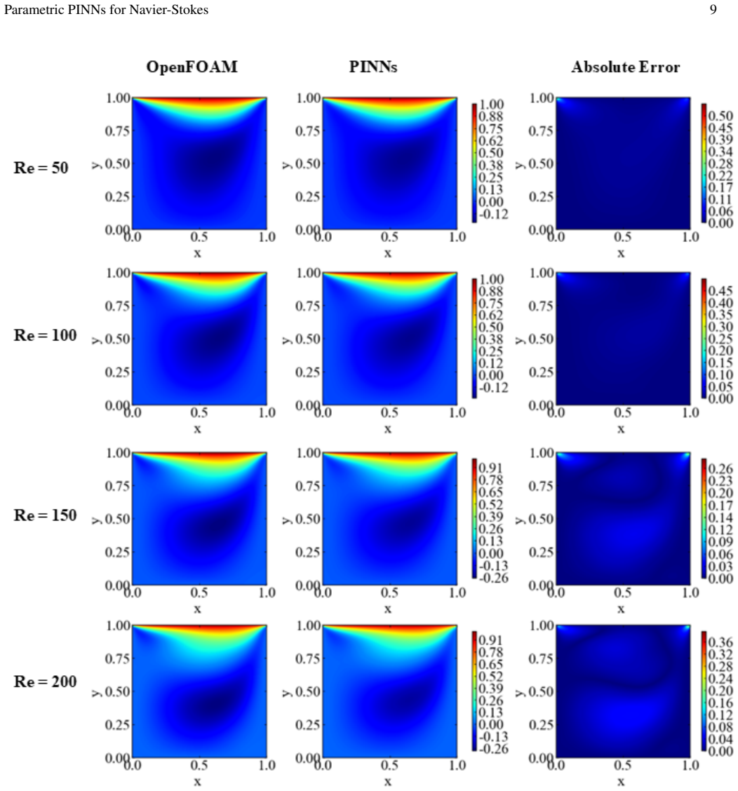
What carries the argument
The central object is a parameterized physics-informed neural network in which the Reynolds number is a third input, log-transformed and normalized so that tanh activations operate in their sensitive regime. The loss is a weighted sum of boundary loss, Navier–Stokes residual loss, and—only in 750<Re<850—a sparse CFD data loss. Training uses Monte Carlo collocation sampling, a two-stage optimizer (stochastic then quasi-Newton), and transfer-learning initialization from a low-Re pure-PINN solution. This combination is what lets the network anchor the high-Re solution manifold with a narrow band of data rather than full coverage.
Load-bearing premise
The accuracy story is measured against a 128×128 uniform-grid finite-volume reference, and the paper treats that reference as effectively exact at every Reynolds number; if that reference under-resolves corner vortices or high-Re boundary layers, every reported MSE and R² value inherits the error, whatever the neural network actually achieved.
What would settle it
Run the identical hybrid training recipe but compare against a grid-converged reference (for instance, a 256×256 or spectral solution) at Re=1000, 1500 and 2000; if the R² values against the coarse reference exceed the agreement between the coarse and the fine reference, the claimed accuracy is an artifact of the reference. A cheaper check is an ablation: remove the data loss entirely at Re=800 and show that R² drops from about 0.998 to below 0.9, confirming the supervision is doing the work claimed.
If this is right
- One trained network replaces per-Reynolds-number CFD solves for steady laminar cavity flow across about Re=500–1000, with usable extrapolation to Re=2000.
- Supervision needs cover only a narrow band of parameter space; at the reported 3–20% point fraction, data-generation cost drops by an order of magnitude or more.
- At low Reynolds numbers the pure physics-only model is sufficient, so a single framework can switch from data-free to data-assisted regimes as convection dominates.
- The parameterization strategy extends to other dimensionless groups, such as Prandtl, Grashof, or Rayleigh numbers, giving surrogate models for families of heat and mass transfer problems.
- Transfer learning from low-Re solutions provides a cheap initialization that stabilizes high-Re training, suggesting a reusable curriculum for parametric PDE solvers.
Where Pith is reading between the lines
- The 5%-data figure should be read as evidence of a principle, not a universal constant: the body never reports the exact number of supervised points or its fraction of the mesh, so the 3–20% and 5% numbers are abstract-level claims that need a reproducibility appendix.
- The abstract promises backward-facing step validation that the body does not contain; until that case is shown with the same 100-wide supervision band, the generality of the method rests on a single geometry.
- Because the reported accuracy peaks inside the data-assisted band, a plausible interpretation is that the data pins down the vortex cores while the PDE residual fills in the rest; testing with the data band moved to 600–650 would reveal whether the anchor is local in parameter space or global across the manifold.
- A harder test is unsteady flow: the current steady-state formulation avoids time-stepping pathologies, so whether the same 5% supervision transfers to time-dependent or three-dimensional flows remains open.
Editorial analysis
A structured set of objections, weighed in public.
Referee Report
Summary. The paper develops a parameterized physics-informed neural network (PINN) for the 2D lid-driven cavity flow, with the Reynolds number as an additional network input. At low Reynolds numbers (Re ≤ 300), a pure physics-only PINN is trained without CFD data and compared against OpenFOAM reference solutions. For higher Reynolds numbers (Re ∈ [500, 1000]), the authors introduce a hybrid framework that adds a sparse CFD data-loss term, with supervision supplied only in the subrange 750 < Re < 850, together with transfer learning from lower-Re models. The reported results include MSE/R² comparisons with OpenFOAM for Re = 200–2000, and the abstract claims that approximately 5% supervised data are sufficient and that the method is validated for backward-facing step flow. The central contribution is a data-efficient, single-network parametric solver that can interpolate and partially extrapolate across Reynolds numbers.
Significance. If the data-efficiency claim were properly established, this would be a practically useful contribution: a single trained network could replace per-Re CFD solves over a range of Reynolds numbers using only a small supervised subset of the parameter space. The manuscript contains several strengths: it uses an external CFD benchmark (OpenFOAM) as reference, reports quantitative metrics (MSE, R²) across many Reynolds numbers, provides convergence and gradient-norm diagnostics, and compares multiple collocation-point sampling strategies. However, the paper's headline quantitative claim — that approximately 5% supervised data are sufficient — is not currently supported by the reported evidence. The key missing pieces are the actual number of supervised points, the loss weights, a data-fraction sweep, and a no-supervision baseline. These are all within the scope of a revision, so the result is plausible but not yet demonstrated.
major comments (3)
- [Abstract; §III.B.1, Eq. (17)] The central claim that "approximately 5% supervised data are sufficient" is not auditable from the reported evidence. Eq. (17) defines the data loss L_D with a normalization by N_D, but N_D is never reported, and the abstract's "3%-20% of computational points" is never connected to any table or experiment. The loss weights λ_b, λ_PDE, λ_D in Eq. (16) are also not listed. No experiment varies the supervised-data fraction, and no N_D = 0 (pure-PINN or transfer-learning-only) baseline is shown for Re ∈ [500, 1000]. Consequently, the high R² values in Table V could be due primarily to the PDE loss and transfer learning rather than to the sparse data term, or alternatively the data term could dominate if λ_D is large. Please report N_D and all loss weights for every case, and add a data-fraction sweep (e.g., 0%, 1%, 3%, 5%, 10%, 20%) to establish the claimed sufficiency of 5% supervision.
- [Abstract; §I and §III] The abstract states that the framework is "further validated for backward-facing step flow," but the full text contains no backward-facing step results, methodology, or even a section devoted to that configuration. The paper is entirely about the lid-driven cavity. This is a claimed validation that is simply absent. Either add the backward-facing step study or remove the claim from the abstract and introduction. The same issue appears in the title of the arXiv metadata, which mentions "Incompressible Flows Across Reynolds Numbers" more broadly than the actual content.
- [§II.A.2 and §III.B.4] All quantitative comparisons use OpenFOAM on a 128×128 grid as ground truth, including extrapolation up to Re = 2000. The manuscript notes that 128×128 resolution is considered sufficient up to approximately Re ≈ 10^3 (citing Erturk et al.), but no grid-convergence or CFD uncertainty study is supplied for Re = 1200, 1500, and 2000. If the CFD reference under-resolves secondary corner vortices or boundary layers at these higher Reynolds numbers, every MSE and R² value in Table V inherits that bias, independent of how well the PINN optimization performed. Please include a grid-refinement check (e.g., 128×128 vs. 256×256 vs. 512×512) for at least the high-Re test cases, or quantify the discretization error of the reference solution.
minor comments (4)
- [§III.A.7 vs. Table IV/V] There is a numbering inconsistency: the low-Reynolds-number section refers to "Table V" when summarizing results that are actually presented in Table IV. The high-Reynolds-number section then uses Table V. Please renumber tables consistently.
- [Eq. (17)] The summation index in Eq. (17) runs to N_d while the denominator is N_D; the notation is inconsistent and should be unified. Also, the definition of N_D as the number of supervised CFD points should be stated explicitly in the text.
- [§III.A.6, Table III] The text states that "the fine grid achieving the best accuracy across all metrics," but at Re = 50 the fine grid has slightly higher MSE (1.96×10⁻⁴) and lower R² (0.9846) than the coarse grid (1.78×10⁻⁴, 0.9860). This is a minor inconsistency; clarify whether the differences are within noise or whether the finest grid is not always strictly best.
- [§III.B.5, Tables VI and VII] The GPU/CPU speedup comparison is confounded: the two tables use different network sizes (H, N), grid sizes, and epoch counts. The claim of a "1.9× speedup" should be based on matched configurations, or the comparison should be explicitly labeled as indicative rather than controlled.
Circularity Check
No significant circularity; the supervised Reynolds-number band is explicitly labeled, and the generalization claims rest on independent evaluation points.
full rationale
The paper's low-Reynolds-number regime is a pure PINNs formulation with no CFD data term, so its agreement with OpenFOAM is an independent external check rather than a fitted prediction. The high-Reynolds-number hybrid model does train on CFD data through Eq. (17), but only within 750<Re<850, and the paper explicitly identifies this band (green-shaded region in Fig. 18, Table V) and does not rely on it as the sole evidence for generalization. Independent evidence is provided at Re=500 and Re=1000 (within the training interval but outside the supervised band) and at Re=1200-2000 (extrapolation), which are not directly fit by the data loss. The abstract's 'approximately 5% supervised data are sufficient' claim is under-supported because ND, lambda_D, and the supervised-point fraction are never reported and no supervision-fraction sweep or zero-data baseline is shown; the promised backward-facing-step validation is also absent. These are reporting and verification gaps, not circular reductions: no equation is shown to be equivalent to its inputs by construction, and the self-citation [27] is a peripheral background reference rather than a load-bearing uniqueness or derivation step. The central parametric-PINN methodology is benchmarked against external OpenFOAM solutions and is not forced by self-citation or by definition.
Axiom & Free-Parameter Ledger
free parameters (4)
- Loss weights λ_b, λ_PDE, λ_D
- Supervised data fraction (3–20% of points, claimed ~5%) =
~5% (reported; exact ND not given)
- Network size (H=10 hidden layers, N=80 neurons per layer) =
10 layers × 80 neurons
- Learning-rate schedule and optimizer switch points =
5e-3 → 1e-6 piecewise schedule
axioms (5)
- domain assumption Steady incompressible Navier-Stokes equations in non-dimensional form (Eqs. 2–5) correctly model the lid-driven cavity up to Re=2000.
- domain assumption OpenFOAM with a 128×128 uniform grid is an accurate reference for all reported Re, including corners and secondary vortices.
- domain assumption A 10-layer tanh feed-forward network with Re as an input can represent the parametric solution manifold accurately enough.
- domain assumption The Adam-then-L-BFGS training procedure actually reaches a low-residual solution that corresponds to the physical Navier-Stokes solution.
- domain assumption Transfer learning from a low-Re pretrained model improves and stabilizes high-Re training sufficiently.
read the original abstract
Physics-informed neural networks (PINNs) provide a mesh-free framework for solving partial differential equations by embedding governing physics into neural-network training. Recent studies have shown that parameterized PINNs can learn Navier-Stokes solutions across Reynolds numbers by treating Reynolds number as an additional network input. However, physics-only PINNs often lose accuracy in convection-dominated high-Reynolds-number flows because of optimization stiffness and multiscale flow structures. This study presents a sparse-supervised hybrid parameterized PINNs framework for incompressible Navier-Stokes flows with regime-aware learning and localized Reynolds-number supervision. The approach is demonstrated for two-dimensional lid-driven cavity flow and further validated for backward-facing step flow. At low Reynolds numbers, physics-only PINNs accurately predict velocity and pressure fields using only governing equations and boundary conditions. At higher Reynolds numbers, sparse CFD supervision combined with transfer learning is introduced to improve predictive accuracy. Although the training range spans (500 < Re < 1000), CFD supervision is applied only within (750 < Re < 850) using just (3%-20%) of computational points. Results show that approximately (5%) supervised data are sufficient for accurate flow prediction. Comparisons with CFD simulations demonstrate strong agreement in velocity, pressure, vorticity, and reattachment characteristics across interpolation and limited extrapolation regimes. The proposed framework provides a practical and data-efficient hybrid strategy for incompressible flows across varying Reynolds numbers.
Figures




Forward citations
Cited by 1 Pith paper
-
Solving Hamiltonian Constraint Equation with Physics-Informed Neural Networks
PINNs with specialized techniques solve the nonlinear Hamiltonian constraint for generic binary black hole initial data, matching traditional NR accuracy.
Reference graph
Works this paper leans on
-
[1]
The computational do- main is a square cavity of dimension 1 × 1
Problem Statement and Boundary Conditions The canonical two-dimensional lid-driven cavity problem is selected as the benchmark test case. The computational do- main is a square cavity of dimension 1 × 1. The top wall (lid) moves with a uniform velocityU lid in the positivexdirection, while the remaining three walls are at no-slip condition. This configura...
-
[2]
Validation of CFD results from existing literature CFD simulations were performed using the open-source finite-volume solverOpenFOAM 12. High-fidelity CFD so- lutions obtained usingOpenFOAMare used as reference data Parametric PINNs for Navier-Stokes 3 for validation.OpenFOAMhas been extensively validated for incompressible laminar cavity flows and is wid...
1993
-
[3]
Neural Network Architecture A fully connected feed-forward neural network (FNN) is employed to approximate the velocity and pressure fields within the cavity, as schematically illustrated in Fig. 2. The network takes three input features: the spatial coordinates (x,y)and the Reynolds number(Re). Treating the Reynolds number as an explicit input parameter ...
-
[4]
Within this domain,N f inte- rior collocation points andN b boundary points are distributed, as illustrated in Fig
Computational Domain The computational domain consists of a two-dimensional square cavity of size 1 × 1. Within this domain,N f inte- rior collocation points andN b boundary points are distributed, as illustrated in Fig. 3. Several sampling strategies were evaluated, including Latin Hypercube sampling, Sobol low- discrepancy sequences, uniform grid sampli...
-
[5]
In the first stage, the Adam optimizer is used to obtain a coarse approximation of the solution, provid- ing suitable initial weights and biases for the network31
Hyperparameters Training of the physics-informed neural network is per- formed in two stages. In the first stage, the Adam optimizer is used to obtain a coarse approximation of the solution, provid- ing suitable initial weights and biases for the network31. In the second stage, the L-BFGS optimizer is employed to further refine convergence and reduce the ...
-
[6]
These weights can be adjusted to balance the relative contributions of each term and prevent any single component from dominating the training process
Loss Function Design The total loss function,L, is defined as a weighted sum of the boundary condition loss and the PDE residual loss: L=λ b Lb +λ PDE LPDE (9) whereλ b andλ PDE are the respective weighting coeffi- cients. These weights can be adjusted to balance the relative contributions of each term and prevent any single component from dominating the ...
-
[7]
The gradient norm measures the overall size of the gradients of each loss term with respect to the train- able parameters of the neural network
Gradient Norm Analysis During the training of PINNs, monitoring the gradient norm is a useful way to evaluate the stability and balance of the op- timization process. The gradient norm measures the overall size of the gradients of each loss term with respect to the train- able parameters of the neural network. Tracking this quantity helps detect common tr...
-
[8]
Each sampling method was trained over the considered range of Reynolds numbers and then tested for the lid-driven cavity flow atRe=100
Effect of Sampling Strategies on PINNs Performance To evaluate the influence of collocation-point sampling strategies on the performance of PINNs, four different meth- ods were examined: Latin Hypercube sampling, Monte Carlo sampling, Sobol low-discrepancy sampling, and a uniform (structured) grid. Each sampling method was trained over the considered rang...
-
[9]
Loss Function Convergence The convergence behavior of the total loss and its individ- ual components is illustrated in Fig. 4. The total loss function consists of contributions from the governing equations (PDE loss) and the boundary conditions (BC loss), with the PDE loss further decomposed into the continuity loss and the mo- mentum losses in thex- andy...
-
[10]
Figure 5 illustrates the variation of the gradient norm with respect to the number of training epochs
Gradient Norm Plot To assess training stability and diagnose stiffness in the optimization process, gradient norm analysis is employed by monitoring the magnitude of gradients associated with differ- ent loss components. Figure 5 illustrates the variation of the gradient norm with respect to the number of training epochs. TABLE II. A piecewise-constant le...
-
[11]
These flow features are consistent with classical numerical and experimental studies of the lid-driven cavity flow1–3,5
Contours ofu,v, andp The predicted velocity and pressure contours reveal the formation of a dominant primary vortex and progressively stronger secondary corner vortices as the Reynolds number increases. These flow features are consistent with classical numerical and experimental studies of the lid-driven cavity flow1–3,5. Parametric PINNs for Navier-Stoke...
-
[12]
Velocity Profiles Velocity profiles along the cavity centerlines are compared with CFD reference solutions following standard valida- tion practices commonly adopted in lid-driven cavity bench- marks2,3. Figure 8 presents a quantitative comparison of velocity pro- files between the PINNs predictions and the CFD reference solutions obtained usingOpenFOAM 1...
-
[13]
Each configura- tion contained both collocation points enforcing the govern- ing equations and boundary points enforcing Dirichlet con- ditions
Influence of Collocation-Point Density on Model Accuracy To assess the sensitivity of the PINNs predictions to the density of training points, three spatial discretizations were employed: a coarse grid (3,300 points), a medium grid (5,200 points), and a fine grid (11,700 points). Each configura- tion contained both collocation points enforcing the govern-...
-
[14]
The Reynolds number range used for model training, 50≤Re≤300, is defined as theinterpola- Parametric PINNs for Navier-Stokes 11 TABLE III
Model Accuracy: Comparison Between CFD and PINNs Predictions To assess both the interpolation and extrapolation capabili- ties of the proposed PINNs framework, the model predictions were compared against high-fidelity CFD solutions at multi- ple Reynolds numbers. The Reynolds number range used for model training, 50≤Re≤300, is defined as theinterpola- Par...
2000
-
[15]
The modified loss function is defined as L=λ b Lb +λ PDE LPDE +λ D LD (16) Parametric PINNs for Navier-Stokes 13 FIG
Loss Function Design for High Reynolds Numbers For high Reynolds number cases, the total loss function is augmented with an additional data-driven term to compen- sate for the dominance of the convective terms in the Navier- Stokes equations. The modified loss function is defined as L=λ b Lb +λ PDE LPDE +λ D LD (16) Parametric PINNs for Navier-Stokes 13 F...
-
[16]
Contours ofu,v, andp Contour plots of the horizontal velocity (u), vertical veloc- ity (v), and pressure (p) fields are presented to visually as- sess the predictive accuracy of the hybrid PINNs framework against high-fidelity CFD reference solutions. The trained PINNs model, informed by sparse CFD data and transfer learning, is used to predict the flow v...
-
[17]
Velocity Profiles Velocity profiles extracted along selected geometric center- lines of the cavity are used to provide a quantitative assess- ment of the predictive accuracy of the hybrid PINNs model. These profiles offer a detailed comparison of the local veloc- ity distributions and serve as strong indicators of the effective- ness of transfer learning ...
-
[18]
The assessment is performed over a wide Parametric PINNs for Navier-Stokes 15 FIG
Model Accuracy: Comparison Between CFD and PINNs Predictions The predictive accuracy of the hybrid PINNs model is quan- titatively evaluated by comparing the predicted velocity and pressure fields with high-fidelity CFD solutions obtained us- ingOpenFOAM 12. The assessment is performed over a wide Parametric PINNs for Navier-Stokes 15 FIG. 13. Comparison ...
2000
-
[19]
Fluid mechanics in the driven cavity,
Loss Function Convergence and GPU Utilization The incorporation of CFD data in the training procedure in- troduces a data loss component alongside the physics-based loss. It is observed that this hybrid loss formulation leads to faster and more stable convergence compared to pure PINNs. The data-driven guidance effectively constrains the solution space, e...
discussion (0)
Sign in with ORCID, Apple, or X to comment. Anyone can read and Pith papers without signing in.