Solving Einstein Field Equations on a Digital Quantum Computer
Pith reviewed 2026-06-26 15:53 UTC · model grok-4.3
The pith
A quantum algorithm evolves the Schwarzschild black hole spacetime and extracts its quasinormal modes on digital quantum hardware.
A machine-rendered reading of the paper's core claim, the machinery that carries it, and where it could break.
Core claim
We develop a proof-of-principle quantum algorithm for solving Einstein Field Equations in the Wahlquist-Estabrook-Buchman-Bardeen (WEBB) tetrad Numerical Relativity formalism, and test it by evolving the Schwarzschild Black Hole spacetime in the WEBB Numerical Relativity formalism, perturbing it to obtain gravitational Quasinormal Modes. We program the algorithm components for a gate-based, digital quantum computer using the Qiskit software and run it on classical simulators and physical IBM quantum computers through the UKRI National Quantum Computing Centre (NQCC) Quantum Access program and quantify the computational resources and runtime.
What carries the argument
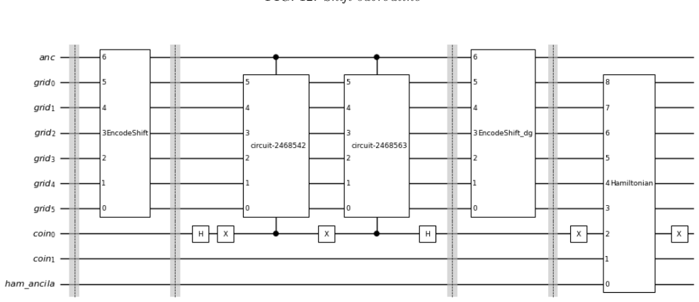
Gate-based quantum circuits that discretize and time-evolve the partial differential equations of the WEBB tetrad formalism for the spacetime metric components.
If this is right
- The unperturbed Schwarzschild metric evolves correctly under the quantum circuit implementation of the WEBB equations.
- Linear perturbations around the black hole produce quasinormal ringing whose frequencies can be read out from the quantum evolution.
- Resource counts for the circuit supply a concrete baseline for estimating the cost of larger grids or longer evolution times.
- Hybrid quantum-classical loops become possible in which the quantum device handles the metric evolution while classical post-processing extracts observables.
Where Pith is reading between the lines
- The same circuit structure could be applied to axisymmetric or rotating black hole backgrounds once the WEBB variables are adapted.
- Error-mitigation layers on present-day hardware might extend the usable evolution time before noise swamps the quasinormal signal.
- Direct side-by-side runs against classical finite-difference codes would reveal whether the quantum representation offers any precision or stability advantage at fixed grid size.
- If device coherence improves, the method might eventually reach regimes near horizons where classical adaptive-mesh codes become expensive.
Load-bearing premise
The chosen discretization and quantum evolution must remain faithful to the continuous WEBB equations without prohibitive accumulation of discretization or hardware noise errors over the grid size and evolution time used.
What would settle it
Run the full circuit on IBM quantum hardware for the perturbed Schwarzschild case and check whether the extracted frequencies of the gravitational quasinormal modes agree with the known analytic values to within the expected hardware error bars.
Figures
read the original abstract
In this work, we show how simulations performed on classical computers such as those of Numerical Relativity can be tackled by quantum algorithms for solving systems of partial differential equations. We develop a proof-of-principle quantum algorithm for solving Einstein Field Equations in the Wahlquist-Estabrook-Buchman-Bardeen(WEBB) tetrad Numerical Relativity formalism [1], and test it by evolving the Schwarzschild Black Hole spacetime in the WEBB Numerical Relativity formalism [2], perturbing it to obtain gravitational Quasinormal Modes [3]. We program the algorithm components for a gate-based, digital quantum computer using the Qiskit software [4] and run it on classical simulators and physical IBM quantum computers through the UKRI National Quantum Computing Centre (NQCC) Quantum Access program and quantify the computational resources and runtime.
Editorial analysis
A structured set of objections, weighed in public.
Referee Report
Summary. The paper claims to develop a proof-of-principle quantum algorithm for solving the Einstein field equations in the Wahlquist-Estabrook-Buchman-Bardeen (WEBB) tetrad numerical relativity formalism. It tests the algorithm by evolving the Schwarzschild black hole spacetime, applying perturbations to extract gravitational quasinormal modes, implements the components in Qiskit, executes them on classical simulators and IBM quantum hardware via the NQCC program, and quantifies the required computational resources and runtime.
Significance. If the central claim were supported by quantitative validation, the work would represent a novel first step toward quantum algorithms for numerical relativity, demonstrating how gate-based quantum computers might address systems of PDEs arising in general relativity. The choice of the WEBB formalism for discretization is a concrete technical decision that could be advantageous for quantum implementation, and the explicit resource quantification is a useful contribution even at the proof-of-principle stage.
major comments (1)
- [Abstract and results section] Abstract and results claims: the manuscript states that the algorithm was programmed and run on IBM quantum computers to evolve the Schwarzschild spacetime and obtain quasinormal modes, yet supplies no quantitative accuracy metrics, error analysis, fidelity measures, or comparison to known analytic QNM frequencies. Without these data it is impossible to assess whether the reported evolution reproduces the target physics or is dominated by discretization and hardware noise, which is load-bearing for the central claim of successful testing.
Simulated Author's Rebuttal
We thank the referee for their constructive feedback and for acknowledging the potential novelty of our approach. We address the major comment point by point below.
read point-by-point responses
-
Referee: [Abstract and results section] Abstract and results claims: the manuscript states that the algorithm was programmed and run on IBM quantum computers to evolve the Schwarzschild spacetime and obtain quasinormal modes, yet supplies no quantitative accuracy metrics, error analysis, fidelity measures, or comparison to known analytic QNM frequencies. Without these data it is impossible to assess whether the reported evolution reproduces the target physics or is dominated by discretization and hardware noise, which is load-bearing for the central claim of successful testing.
Authors: We agree with the referee that quantitative validation is crucial for supporting the claims made in the abstract and results. The current version presents the algorithm development and initial executions as a proof-of-principle, with the hardware component focused on demonstrating implementability rather than precise physics reproduction. To address this, we will revise the manuscript to include fidelity metrics from the simulator runs, an error analysis for the discretization, and a comparison of the obtained QNM frequencies to analytic values. We will also temper the language in the abstract regarding the hardware results to reflect the limitations due to noise, making the scope of the testing clearer. These changes will be incorporated in the revised version. revision: yes
Circularity Check
No significant circularity; new quantum algorithm implementation is self-contained
full rationale
The paper presents a constructive proof-of-principle quantum algorithm for discretizing and evolving the WEBB tetrad PDE system on gate-based hardware, implemented in Qiskit and tested via simulation and IBM runs on the known Schwarzschild background with added perturbations to extract QNMs. No load-bearing step reduces by definition or construction to its own inputs: the algorithm components are specified independently, the test case uses an external known solution rather than a fitted parameter relabeled as prediction, and citations to the WEBB formalism and QNM literature are external references rather than self-citation chains that justify uniqueness or force the result. The derivation chain consists of standard quantum simulation techniques applied to an established NR system and is therefore self-contained against external benchmarks.
Axiom & Free-Parameter Ledger
Reference graph
Works this paper leans on
-
[1]
increase
Quasinormal modes Quasinormal modes (QNMs) are the resonant frequen- cies of a perturbed black hole[69–71], with frequencies and damping determined solely by the black hole param- eters. The Regge-Wheeler (Φ m ℓ ) and Zerilli (Ψ m ℓ ) func- tions govern the odd and even parity sectors of metric perturbations respectively, and obey □Φm ℓ −V RWΦm ℓ = 0 □Ψm ...
-
[2]
Carleman linearisation
-
[3]
local linearisation through the Jacobian matrix of S(q)
-
[4]
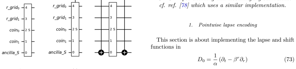
heuristic collision operator; We give more details of each method in the Appendix section B. For this proof-of-principle implementation of the algorithm, we tested the Jacobian and heuristic col- lision operators and checked that they provide similar results (notice figure 15 shows the result obtained from the heuristic collision operator in the Appendix,...
-
[5]
The amplitude- encoding relation is given by Uencode =R y (θr)|0⟩ a|r⟩= ( p 1−p r|0⟩a + √pr|1⟩a)|r⟩ (74) where|r⟩=|x 0
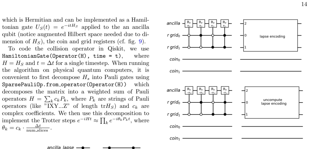
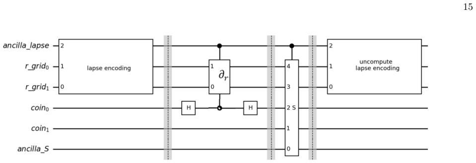
Pointwise lapse encoding This section is about implementing the lapse and shift functions in D0 = 1 α (∂t −β r∂r) (73) A fixed lapse functionα r can be amplitude-encoded in an ancilla qubit through controlledR y(θr) rotations con- ditioned on the spatial grid register. The amplitude- encoding relation is given by Uencode =R y (θr)|0⟩ a|r⟩= ( p 1−p r|0⟩a +...
-
[6]
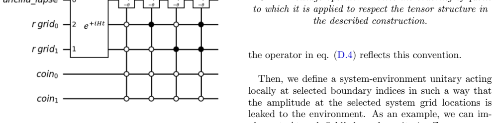
Disentangling the ancilla from the grid register as explained in the next section reduces entanglement-induced mixing effects when tracing out the ancilla and is hence advised
Condition operations on lapse ancilla qubit Conditioning operations onq a =|1⟩ a now induces an αr-dependent weighting in the reduced dynamics after tracing out or postselecting the ancilla. Disentangling the ancilla from the grid register as explained in the next section reduces entanglement-induced mixing effects when tracing out the ancilla and is henc...
-
[7]
To disentangle it, we applyU † encode which amounts to applying the same subroutine as before with negative angles (cf
Uncomputing the lapse encoding Notice that at this pointq a is still entangled with the grid qubits. To disentangle it, we applyU † encode which amounts to applying the same subroutine as before with negative angles (cf. fig. 10). To code the lapse encoding step in Qiskit, we build the subcircuit shown in fig.10 and then wrap it into an In- struction obje...
-
[8]
conditioned on coin1 =|0⟩and coin 1 =|1⟩as it needs to be to all fields equally
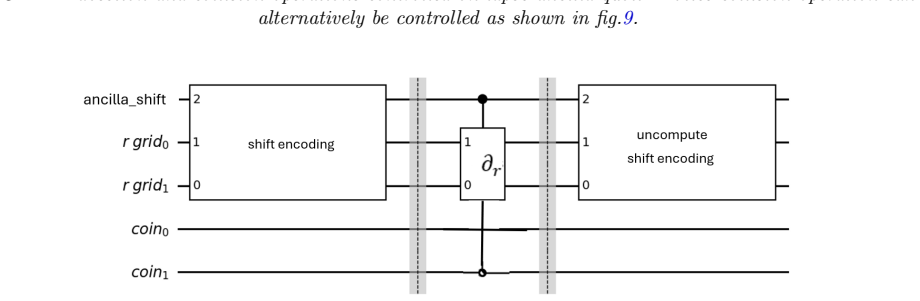
Static shift The subroutine to implement a shiftβ r∂r with a static shift functionβ r is the same as for the lapse, but the derivative∂ r is implemented with either the increase or decrease operator (fig.8) depending on the direction, and controlled as shown in fig.(12), i.e. conditioned on coin1 =|0⟩and coin 1 =|1⟩as it needs to be to all fields equally....
-
[9]
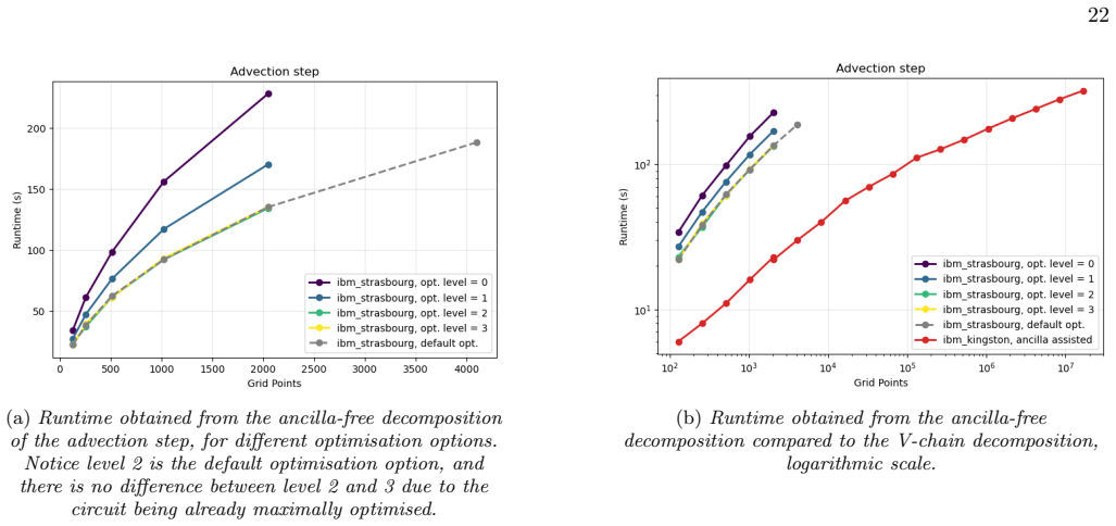
Experiment method Once the circuit is defined and the physical backend is selected, the circuit is transformed in a set of instruc- tions for the backend to execute throughtranspiling: this process includes converting high level gates (e.g. Toffoli, custon unitary gates, etc.) into the device’s native gates, mapping logical qubits in the circuit to physic...
-
[10]
TheV-chainmethod uses a singly controlled V gate (such thatV 2 =U) and CNOT gates, which are recursively applied to different controls, creating a chain of intermediate controls
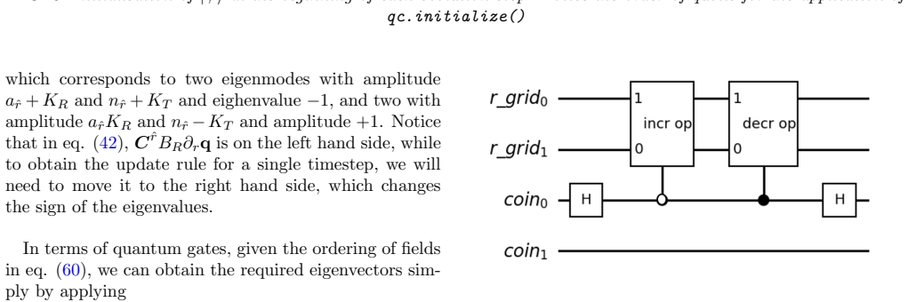
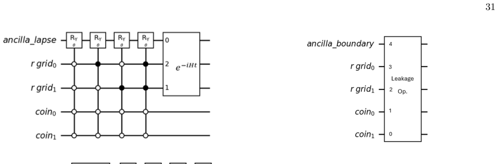
Operations decomposition: advection Multiply controlled gates such as those in the ad- vection and lapse encoding steps can be synthesised in different ways with different resulting runtimes. TheV-chainmethod uses a singly controlled V gate (such thatV 2 =U) and CNOT gates, which are recursively applied to different controls, creating a chain of intermedi...
-
[11]
as a se- quence of controlledR y rotations arranged in a multi- plexed structure
Operations decomposition: lapse encoding The lapse encoding/decoding step has the structure of auniformly controlled rotation (UCRY), i.e. as a se- quence of controlledR y rotations arranged in a multi- plexed structure. UCRY (θ0, . . . , θ2k−1) = 2k−1X i=0 |i⟩⟨i| ⊗R y (θi) (77) This belongs to the more general category of aquan- tum multiplexer, which ca...
-
[12]
(81) where the coefficientsc j are real numbers,P j is a tensor product of Pauli matrices (e.g.,I, X, Y, Z) which forms a complete operator basis
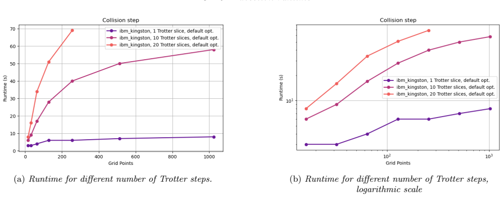
Operations decomposition: collision operator A Hamiltonian acting onnqubits can bePauli- decomposedas H= MX j=1 cjPj = X j cj P (1) j ⊗P (2) j ⊗ · · · ⊗P (n) j . (81) where the coefficientsc j are real numbers,P j is a tensor product of Pauli matrices (e.g.,I, X, Y, Z) which forms a complete operator basis. While the computational cost for a general dense...
-
[13]
Regarding the measurement after each step, we want to measure|ψ⟩in the computational basis
Measurement and potential bottlenecks Notice that the state-preparation for structured or con- tinuous functions (as is the case here) can be shown to scale asO(poly(n) and not provide a dramatic increasing in the runtime. Regarding the measurement after each step, we want to measure|ψ⟩in the computational basis. Running the circuitNtimes (”shots”) lets u...
-
[14]
This is because the error due to decoding would likely be larger than the error due to not disentangling the ancilla
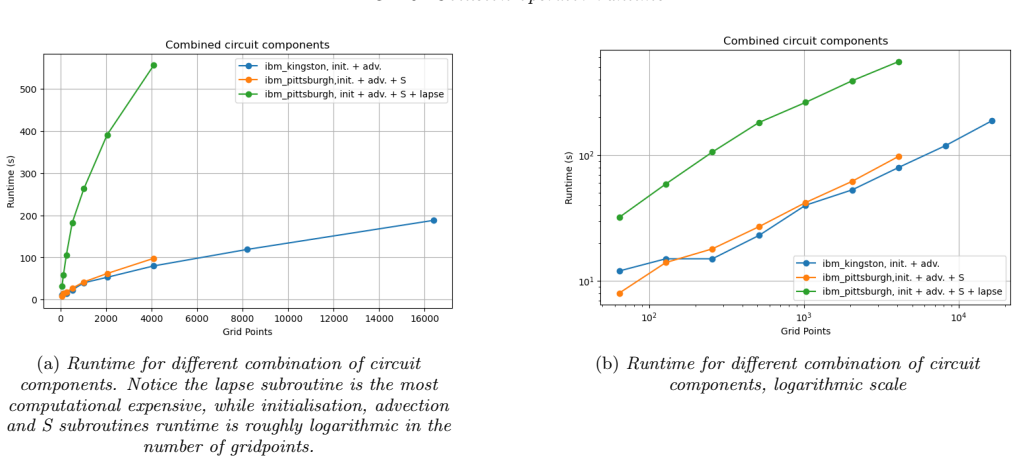
Experiments The runs on physical backends in fig.18 can be divided into three groups: •most recent runs: where we used the circuit in fig.(13) without the lapse decoding step. This is because the error due to decoding would likely be larger than the error due to not disentangling the ancilla. We assign the additional ancillas due to the v-chain decomposit...
-
[15]
Concepts of Quantum and Spacetime
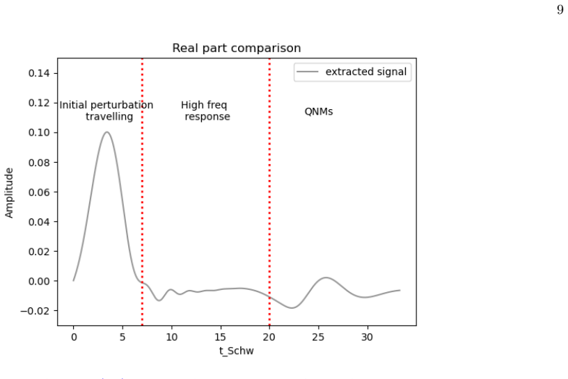
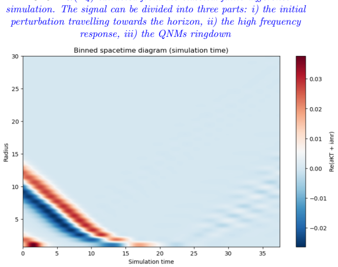
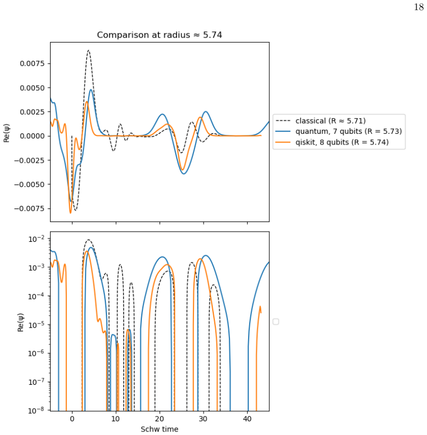
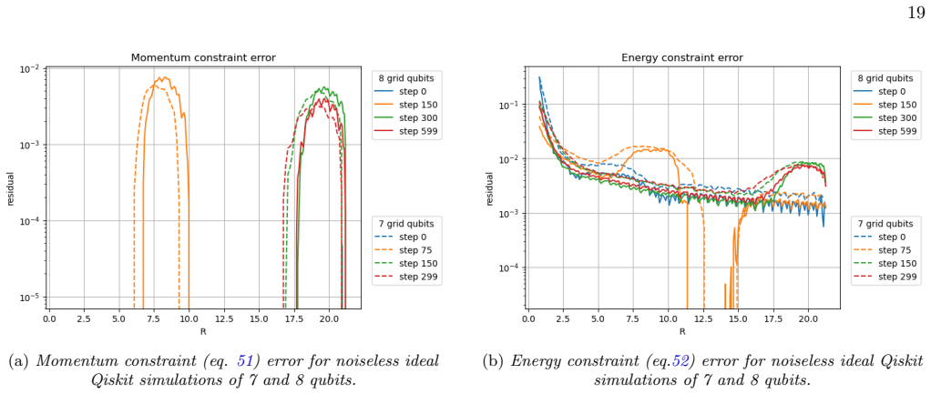
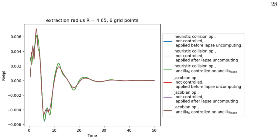
Noise and signal extraction We first tried to extract the QNMs frequencies by fit- ting the signals obtained from the unfiltered noisy simula- tions, and then by applying a moving average smoothing method to i) only the space domain, ii) only the time do- main, iii) both space and time domains (cf. fig.??, where to obtain a better signal to noise ratio we...
2026
-
[16]
M. A. Nielsen and I. L. Chuang, Quantum Com- putation and Quantum Information (2012), 10.1017/cbo9780511976667
-
[17]
Quantum com- plexity vs classical complexity: A survey,
A. Vaezi, A. Movaghar, M. Ghodsi, S. M. H. Kazemi, N. B. Noghrehy, and S. M. Kazemi, “Quantum com- plexity vs classical complexity: A survey,” (2024), arXiv:2312.14075 [cs.CC]
arXiv 2024
-
[18]
Y. Kim, A. Eddins, S. Anand, K. X. Wei, E. van den Berg, S. Rosenblatt, H. Nayfeh, Y. Wu, M. Zaletel, K. Temme, and A. Kandala, Nature618, 500 (2023)
2023
-
[19]
Noisy intermediate-scale quantum algorithms,
K. Bharti, A. Cervera-Lierta, T. H. Kyaw, T. Haug, S. Alperin-Lea, A. Anand, M. Degroote, H. Heimonen, J. S. Kottmann, T. Menke, W.-K. Mok, S. Sim, L.- C. Kwek, and A. Aspuru-Guzik, Reviews of Modern Physics94(2022), 10.1103/revmodphys.94.015004
-
[20]
D. E. Deutsch, A. Barenco, and A. Ekert, Proceedings of the Royal Society of London. Series A: Mathematical and Physical Sciences449, 669–677 (1995)
1995
-
[21]
Barenco, C
A. Barenco, C. H. Bennett, R. Cleve, D. P. DiVincenzo, N. Margolus, P. Shor, T. Sleator, J. A. Smolin, and H. Weinfurter, Physical Review A52, 3457–3467 (1995)
1995
-
[22]
Z. Meng and Y. Yang, Physical Review Research5 (2023), 10.1103/physrevresearch.5.033182
-
[23]
Lewis, S
D. Lewis, S. Eidenbenz, B. Nadiga, and Y. Suba¸ sı, Quantum8, 1509 (2024)
2024
-
[24]
L. Ruiz-Perez and J. C. Garcia-Escartin, Quantum In- formation Processing16(2017), 10.1007/s11128-017- 1603-1
-
[25]
Op- timizing quantum circuits for arithmetic,
T. H¨ aner, M. Roetteler, and K. M. Svore, “Op- timizing quantum circuits for arithmetic,” (2018), arXiv:1805.12445 [quant-ph]
Pith/arXiv arXiv 2018
-
[26]
Quantum implementation of el- ementary arithmetic operations,
G. Florio and D. Picca, “Quantum implementation of el- ementary arithmetic operations,” (2004), arXiv:quant- ph/0403048 [quant-ph]
arXiv 2004
-
[27]
Reversible addition circuit using one ancillary bit with application to quantum computing,
P. Kaye, “Reversible addition circuit using one ancillary bit with application to quantum computing,” (2004), arXiv:quant-ph/0408173 [quant-ph]
Pith/arXiv arXiv 2004
-
[28]
Vedral, A
V. Vedral, A. Barenco, and A. Ekert, Physical Review A54, 147–153 (1996)
1996
-
[29]
Takahashi and N
Y. Takahashi and N. Kunihiro, Quantum Information and Computation5, 440–448 (2005)
2005
-
[30]
Arithmetic circuits for quantum computing: A software library,
L. Raggi, “Arithmetic circuits for quantum computing: A software library,” (2020)
2020
-
[31]
Addition on a quantum computer,
T. G. Draper, “Addition on a quantum computer,” (2000), arXiv:quant-ph/0008033 [quant-ph]
Pith/arXiv arXiv 2000
-
[32]
Shor, inProceedings 35th Annual Symposium on Foundations of Computer Science(1994) pp
P. Shor, inProceedings 35th Annual Symposium on Foundations of Computer Science(1994) pp. 124–134
1994
-
[33]
An approximate fourier transform useful in quantum factoring,
D. Coppersmith, “An approximate fourier transform useful in quantum factoring,” (2002), arXiv:quant- ph/0201067 [quant-ph]
arXiv 2002
-
[35]
D. Reitzner, D. Nagaj, and V. Buˇ zek, Acta Physica Slo- vaca. Reviews and Tutorials61(2011), 10.2478/v10155- 011-0006-6
-
[36]
Fillion-Gourdeau and E
F. Fillion-Gourdeau and E. Lorin, Numerical Algo- rithms82, 1009–1045 (2018)
2018
-
[37]
Quantum com- putation of fluid dynamics,
S. S. Bharadwaj and K. R. Sreenivasan, “Quantum com- putation of fluid dynamics,” (2020), arXiv:2007.09147 [quant-ph]
arXiv 2020
-
[38]
Y. Cao, A. Papageorgiou, I. Petras, J. Traub, and S. Kais, New Journal of Physics15, 013021 (2013)
2013
-
[39]
A. J. Pool, A. D. Somoza, M. Lubasch, and B. Horstmann, 2022 IEEE International Conference on Quantum Computing and Engineering (QCE) (2022), 10.1109/qce53715.2022.00146
-
[40]
Quantum vs. classical algorithms for solving the heat equation,
N. Linden, A. Montanaro, and C. Shao, “Quantum vs. classical algorithms for solving the heat equation,” (2020), arXiv:2004.06516 [quant-ph]
arXiv 2020
-
[41]
D. W. Berry, Journal of Physics A: Mathematical and Theoretical47, 105301 (2014)
2014
-
[43]
Carleman linearization of partial differen- tial equations,
T. Vaszary, “Carleman linearization of partial differen- tial equations,” (2024), arXiv:2412.00014 [math.GM]
arXiv 2024
-
[44]
A. M. Childs, J.-P. Liu, and A. Ostrander, Quantum 5, 574 (2021)
2021
-
[45]
A theory of quantum differential equation solvers: limitations and fast-forwarding,
D. An, J.-P. Liu, D. Wang, and Q. Zhao, “A theory of quantum differential equation solvers: limitations and fast-forwarding,” (2023), arXiv:2211.05246 [quant-ph]
arXiv 2023
-
[46]
J´ oczik, Z
S. J´ oczik, Z. Zimbor´ as, T. Majoros, and A. Kiss, Ap- plied Sciences12, 2873 (2022)
2022
-
[47]
Quantum simulation of partial differential equations via schrodingerisation,
S. Jin, N. Liu, and Y. Yu, “Quantum simulation of partial differential equations via schrodingerisation,” (2022), arXiv:2212.13969 [quant-ph]
arXiv 2022
-
[48]
Quantum simulation of par- tial differential equations via schrodingerisation: tech- nical details,
S. Jin, N. Liu, and Y. Yu, “Quantum simulation of par- tial differential equations via schrodingerisation: tech- nical details,” (2022), arXiv:2212.14703 [quant-ph]
arXiv 2022
-
[49]
R. Demirdjian, D. Gunlycke, C. A. Reynolds, J. D. Doyle, and S. Tafur, Quantum Information Processing 21(2022), 10.1007/s11128-022-03667-7
-
[50]
Qade: Solving dif- ferential equations on quantum annealers,
J. C. Criado and M. Spannowsky, “Qade: Solving dif- ferential equations on quantum annealers,” (2022), arXiv:2204.03657 [quant-ph]
arXiv 2022
-
[51]
L. T. Buchman and J. M. Bardeen, Physical Review D 67(2003), 10.1103/physrevd.67.084017
-
[52]
Arnowitt, S
R. Arnowitt, S. Deser, and C. W. Misner, General Rel- ativity and Gravitation40, 1997–2027 (2008)
1997
-
[53]
T. W. Baumgarte and S. L. Shapiro,Numerical relativ- ity: Solving einstein’s equations on the computer(Cam- bridge University Press, 2010)
2010
-
[54]
Alcubierre,Introduction to 3+1 numerical relativity (Oxford University Press, 2008)
M. Alcubierre,Introduction to 3+1 numerical relativity (Oxford University Press, 2008)
2008
-
[55]
Pretorius, Classical and Quantum Gravity22, 425–451 (2005)
F. Pretorius, Classical and Quantum Gravity22, 425–451 (2005). 25
2005
-
[56]
Lindblom, M
L. Lindblom, M. A. Scheel, L. E. Kidder, R. Owen, and O. Rinne, Classical and Quantum Gravity23, S447–S462 (2006)
2006
-
[57]
Solving systems of linear equa- tions: Hhl from a tensor networks perspective,
A. M. Ali, I. P. Delgado, M. R. Roura, A. M. F. de Lec- eta, and S. V. Romero, “Solving systems of linear equa- tions: Hhl from a tensor networks perspective,” (2026), arXiv:2309.05290 [quant-ph]
Pith/arXiv arXiv 2026
-
[59]
S. Bernuzzi and D. Hilditch, Physical Review D81 (2010), 10.1103/physrevd.81.084003
-
[60]
Anderson and J
A. Anderson and J. W. York, Physical Review Letters 82, 4384–4387 (1999)
1999
-
[61]
Newman and R
E. Newman and R. Penrose, Journal of Mathematical Physics3, 566–578 (1962)
1962
-
[64]
S. Succi, F. Fillion-Gourdeau, and S. Palpacelli, EPJ Quantum Technology2(2015), 10.1140/epjqt/s40507- 015-0025-1
-
[65]
Sbragaglia, R
M. Sbragaglia, R. Benzi, L. Biferale, S. Succi, K. Sugiyama, and F. Toschi, Phys. Rev. E75, 026702 (2007)
2007
-
[66]
Gabbanelli, G
S. Gabbanelli, G. Drazer, and J. Koplik, Phys. Rev. E 72, 046312 (2005)
2005
-
[67]
P. J. Ollitrault, A. Miessen, and I. Tavernelli, Accounts of Chemical Research54, 4229–4238 (2021)
2021
-
[68]
Holmes, N
Z. Holmes, N. J. Coble, A. T. Sornborger, and Y. b. u. Suba¸ s ı, Phys. Rev. Res.5, 013105 (2023)
2023
-
[69]
A quantum algo- rithm to solve nonlinear differential equations,
S. K. Leyton and T. J. Osborne, “A quantum algo- rithm to solve nonlinear differential equations,” (2008), arXiv:0812.4423 [quant-ph]
Pith/arXiv arXiv 2008
-
[70]
Geraldi, S
A. Geraldi, S. De, A. Laneve, S. Barkhofen, J. Sperling, P. Mataloni, and C. Silberhorn, Phys. Rev. Res.3, 023052 (2021)
2021
-
[71]
Collision Models Can Efficiently Simulate Any Multipartite Markovian Quantum Dynamics
M. Cattaneo, G. De Chiara, S. Maniscalco, R. Zambrini, and G. L. Giorgi, Physical Review Letters126(2021), 10.1103/physrevlett.126.130403
-
[72]
An efficient quantum algorithm for the one- dimensional burgers equation,
J. Yepez, “An efficient quantum algorithm for the one- dimensional burgers equation,” (2002), arXiv:quant- ph/0210092 [quant-ph]
arXiv 2002
-
[73]
A. Mezzacapo, M. Sanz, L. Lamata, I. L. Egusquiza, S. Succi, and E. Solano, Scientific Reports5(2015), 10.1038/srep13153
-
[74]
Burger, L
A. Burger, L. C. Kwek, and D. Poletti, Entropy24, 1766 (2022)
2022
-
[75]
He and L.-S
X. He and L.-S. Luo, Physical Review E56, 6811–6817 (1997)
1997
-
[76]
Succi and R
S. Succi and R. Benzi, Physica D: Nonlinear Phenomena 69, 327–332 (1993)
1993
-
[77]
B. L. Douglas and J. B. Wang, Physical Review A79 (2009), 10.1103/physreva.79.052335
-
[78]
F. Fillion-Gourdeau, H. J. Herrmann, M. Mendoza, S. Palpacelli, and S. Succi, Physical Review Letters 111(2013), 10.1103/physrevlett.111.160602
-
[79]
SUZUKI, Proceedings of the Japan Academy, Series B69, 161–166 (1993)
M. SUZUKI, Proceedings of the Japan Academy, Series B69, 161–166 (1993)
1993
-
[80]
O. Sarbach and M. Tiglio, Physical Review D64(2001), 10.1103/physrevd.64.084016
-
[81]
L. T. Buchman and O. C. A. Sarbach, Classical and Quantum Gravity24, S307–S326 (2007)
2007
-
[82]
L. T. Buchman and J. M. Bardeen, Physical Review D 72(2005), 10.1103/physrevd.72.124014
-
[83]
J. M. Nester, Journal of Mathematical Physics33, 910–913 (1992)
1992
-
[84]
L. Sberna, P. Bosch, W. E. East, S. R. Green, and L. Lehner, Physical Review D105(2022), 10.1103/physrevd.105.064046
-
[86]
K. D. Kokkotas and B. G. Schmidt, Living Reviews in Relativity2(1999), 10.12942/lrr-1999-2
discussion (0)
Sign in with ORCID, Apple, or X to comment. Anyone can read and Pith papers without signing in.