REVIEW 4 major objections 4 minor 26 references
Parameter Robustness in Data-Driven Estimation of Dynamical Systems
T0 review · 4 major / 4 minor · reviewed 2026-08-04 · deepseek-v4-flash
Pith's one-line read The sensitivity of estimation error to each parameter is bounded by an explicit formula, so robustness can be checked without simulation.
desk verdict The paper has a clean framework and a correct unforced special case, but the headline forced-input bound fails on a simple input-scaling argument and the proof mixes norms and horizons. read the letter →
The pith
A machine-rendered reading of the paper's core claim, the machinery that carries it, and where it could break.
The reading
What carries the argument
The load-bearing object is the augmented error system, x̄ = [x; x̃], Ā = diag(A, Ã), B̄ = [B; B̃], C̄ = C − C̃, whose output ȳ is exactly the estimation error. The proof machinery is a pair of derivative bounds for matrix exponentials: Lemma 2 bounds ‖∂e^{At}/∂θ_i‖ by ‖∂A/∂θ_i‖ t e^{-|µ|t} for Hurwitz A, and Lemma 3 bounds the negative-time exponential e^{-As} similarly. These turn the sensitivity integral into moments of t against decaying exponentials, which produce the explicit constants 1/(4|µ|³), 2/|µ|⁵, and 2/|µ|, and hence K1, K2, K3. The log-norm µ = λmax(Ā+Āᵀ)/2 encodes the stability margin, so the constants reflect how quickly the augmented error system forgets both initial conditi
What would settle it
Pick a Hurwitz but poorly conditioned A(θ), compute ||∂e^{At}/∂θ|| numerically by finite differences over a grid of t up to horizon N, and check whether it ever exceeds ||∂A/∂θ|| t e^{-|mu|t}. Alternatively, simulate the mass-spring-damper LPV example with the paper's parameters, compute ∂ȳ/∂θ₁ by finite differences, and compare its squared 2-norm to the Theorem 1 bound; any violation of the bound at a single t would refute the central claim.
Extended reading notes
Core claim
The central claim is Theorem 1: for the augmented error system ẋ̄ = Āx̄ + B̄u, ȳ = C̄x̄ with Ā block diagonal containing A and the estimated Ã, the squared 2-norm of the sensitivity ∂ȳ/∂θ_i is bounded by K1 ‖∂Ā/∂θ_i‖² + K2 ‖∂Ā/∂θ_i‖³ ‖B̄u‖∞ + K3 N² ‖∂Ā/∂θ_i‖² ‖B̄u‖∞, with K1, K2, K3 given explicitly in terms of the augmented output matrix, initial condition, log-norm, and horizon. The bound is assembled from the convolution solution of the augmented system; the key move is to pass derivatives through the matrix exponential and apply Lemmas 2 and 3, which bound ‖∂e^{At}/∂θ_i‖ ≤ ‖∂A/∂θ_i‖ t e^{-|µ|t} (and its negative-time analogue) for Hurwitz A. Each of the four products from expanding the s
Load-bearing premise
The load-bearing premise is that Lemma 2's uniform bound ||∂e^{At}/∂θ_i|| ≤ ||∂A/∂θ_i|| t e^{-|mu|t} holds for every matrix argument and every time in the convolution integrals, including negative-time exponentials; the K1, K2, K3 constants come from integrating that decay, so a counterexample to the bound would break the formula.
Editorial extensions
If this is right
- Estimator selection can be made parameter-aware: for each θ_i, compute the Theorem 1 bound on the augmented system and rank candidate estimators on sensitivity to that parameter.
- The robustness metric R can be restricted to a subset of physically relevant parameters, isolating, say, motor constants or aerodynamic coefficients in a rotor system while ignoring others.
- The unforced-input special case reproduces the known model-reduction robustness bound, and the zero-initial-condition case gives K3N²‖∂Ā/∂θ_i‖²‖B̄u‖∞; both validate the theorem as an extension rather than a separate result.
- For parameter-dependent initial conditions, Theorem 2 gives a bound through the maximum eigenvalue of the observability Gramian P, again computable without trajectory simulation.
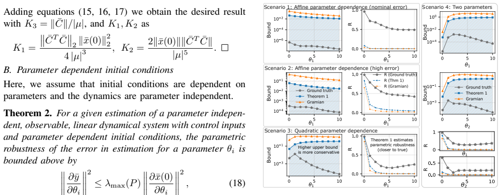
- The LPV mass-spring-damper example indicates the new bound is tighter than a finite-horizon observability-Gramian bound, making it usable as a worst-case guarantee rather than merely a formal one.
Reading between the lines
- The proof is written for parameter dependence in A and x(0); the same convolution expansion with ∂B̄/∂θ_i and ∂C̄/∂θ_i terms would extend Theorem 1 to fully parameter-dependent B and C, an extension the paper leaves implicit.
- Because K1 and K2 scale as 1/|µ|³ and 1/|µ|⁵, near-marginal systems will make the bound conservative; a finite-horizon analogue might trade tightness for practical usability.
- One can test the metric's utility directly: on a benchmark parameterized system, compare the Theorem 1 sensitivity ranking across estimators with rankings from finite-difference ground truth; the paper motivates but does not run that benchmark.
- Reading R as a cost function opens a design loop — choose estimated parameters to maximize R with respect to nuisance parameters while keeping sensitivity to parameters of interest high; the paper names this direction as future work.
Editorial analysis
A structured set of objections, weighed in public.
Referee Report
Summary. The paper proposes a sensitivity-based robustness metric for the estimation error of parameterized linear dynamical systems with control inputs. The central object is the augmented error system of Eqs. (5)-(7), and the robustness metric R in Eqs. (4)/(9) is defined through the normalized sensitivity of the estimation error. The main theoretical contribution is Theorem 1 (Eq. (13)), which claims a trajectory-free upper bound on the squared norm of the sensitivity ∂ȳ/∂θ_i in terms of ‖∂Ā/∂θ_i‖, the input norm ‖B̄u‖∞, and constants K1,K2,K3 involving the initial condition, the log-norm of Ā, C̄, and a horizon N. Theorem 2 handles parameter-dependent initial conditions. The paper also includes an LPV mass-spring-damper example and a comparison with a Gramian-based bound. The u=0 special case (Eq. (20)) reproduces a bound from the author's prior model-reduction work.
Significance. If Theorem 1 were correct, it would give a useful, easily computable certificate of parametric robustness for data-driven estimators, avoiding repeated simulation. A notable strength is the explicit claim of a closed-form bound and the availability of code. The u=0 reduction to existing results provides a partial consistency check. However, the forced-input extension, which is the paper's main novelty, is unsound: the claimed inequality has the wrong scaling in input amplitude, and the quantity bounded in the proof is an L2 norm that is not connected to the pointwise robustness metric R defined in Section II. Since these are foundational to the paper's central claim, the contribution is not established.
major comments (4)
- [Section IV.A, Theorem 1, Eq. (13)] The LHS of Eq. (13) is defined in the proof as ∫_0^∞ ‖∂ȳ/∂θ_i(t)‖^2 dt, i.e., the squared L2 norm of the sensitivity. Differentiating Eq. (14) shows u ↦ ∂ȳ/∂θ_i is affine, with forced-response part linear in u. Replacing u by c u scales the forced part of the LHS by c^2, while the RHS's K2 and K3 terms scale only by c. For any input direction with nonzero forced sensitivity, the RHS/LHS ratio tends to zero as c→∞, so Eq. (13) cannot hold. The same defect appears in Eq. (15), where a1b2 is a squared norm but is bounded by a term linear in ‖B̄u‖∞. This is not a question of conservatism; it is a scaling contradiction.
- [Section II.B and Section IV.A] The metric R in Eqs. (4) and (9) is defined pointwise in time through the ratio ‖∂err/∂θ_i(t)‖ / ‖err(t)‖. Theorem 1 instead bounds the time-integrated quantity ∫_0^∞ ‖∂ȳ/∂θ_i(t)‖^2 dt. The paper does not prove that this L2 bound controls the pointwise ratios appearing in R, nor does it define the norm in Eq. (13) consistently with the pointwise norm used in the metric. Thus, even setting aside the scaling issue, the theorem does not establish the advertised robustness metric.
- [Section IV.A, Eqs. (13)-(15)] The LHS of Eq. (13) is an integral over [0,∞), while K3 contains N^2, where N is described as the maximum time for which inputs are applied. If a finite horizon was intended, the theorem should state the LHS as ‖∂ȳ/∂θ_i‖_{2,[0,N]}^2 and all intermediate bounds (e.g., Eq. (15)) should be derived on [0,N]; if an infinite horizon was intended, the N^2 term is undefined. The proof of Eq. (15) integrates to ∞ and then introduces N ad hoc, so the theorem's time horizon is not well defined.
- [Appendix A, a2b2 bound] The derivation of the a2b2 term replaces the inner integral ∫_0^t C̄ ∂e^{Ā(t-τ)}/∂θ_i B̄u(τ)dτ by ∫_0^t ∂e^{-Āτ}/∂θ_i B̄u(τ)dτ. These are not equal: ∂e^{A(t-τ)}/∂θ_i is not the derivative of e^{-Aτ}. The subsequent use of Lemma 3 is therefore applied to a different integral, and the K2 contribution in Eq. (17) is not established. A demonstration that the replacement is a valid conservative bound is needed.
minor comments (4)
- [Section II.B, Eq. (3)] The typesetting of d_R is garbled; the placement of absolute-value bars and the division structure are unclear. Please rewrite the definition with clear parentheses.
- [Section II.A] The statement that D=0 is 'without loss of generality' needs a concrete explanation of how the D term is incorporated. As written, Theorems 1 and 2 assume D=0, but the augmented system definition (6) includes D̄.
- [Section III, Lemma 1] Lemma 1 states a bound for e^{At} without specifying the time domain. Lemma 3 applies the same type of estimate to negative-time arguments; a two-sided log-norm bound and its domain of validity should be stated explicitly.
- [Section V, Figures 1-2] The figures lack axis labels and units. The statement that the proposed bound is 'closer to true' would be easier to assess if the ground-truth norm, the baseline Gramian norm, and the time horizon were clearly specified.
Circularity Check
No significant circularity: Theorem 1 is derived from standard convolution identities and decay bounds, not fitted or defined into existence.
full rationale
The paper's central result, Theorem 1, is obtained by writing the augmented output as a convolution expression (eq. 14), differentiating with respect to a parameter, expanding the product into four terms, and bounding each with Lemma 2 / Lemma 3 plus the logarithmic-norm decay estimate of Lemma 1. These lemmas are proved from the standard integral representation of the derivative of a matrix exponential, with no hidden use of the theorem being proved. The robustness metric in eqs. (3)-(4) is a definition adapted from the author's prior work [21] and is not used as an input to force the bound; it merely names the quantity that the theorem bounds. The self-citations to [21] and [26] appear in the special-case validation (eqs. 19-21) and in Theorem 2's proof method, but the forced-input bound does not depend on those results for its derivation. There is no fitted parameter renamed as a prediction, no uniqueness theorem imported from the authors, and no ansatz smuggled in via citation. The u=0 and x(0)=0 special cases are consistency checks, not load-bearing assumptions. Any mathematical concerns about Lemma 2/3 or the scaling of the bound are correctness issues, not circularity: the derivation is self-contained and the claimed inequality is not equivalent by definition to its own inputs.
Assumptions & free parameters
free parameters (1)
- N (finite time horizon) =
user-specified, not fixed in the paper
assumptions (6)
- domain assumption Both true and estimated systems are exponentially stable and ISS stable.
- domain assumption The estimated system has the same parameterized structure as the true system.
- domain assumption D = 0 without loss of generality.
- standard math Lemma 1 (log-norm bound): for Hurwitz A, ||e^{At}|| <= e^{-|mu|t}.
- ad hoc to paper Lemma 2/3 derivative bounds apply uniformly to the matrix exponentials inside the convolution integrals, including e^{-A tau}.
- domain assumption The augmented system (Abar,Cbar) is observable in Theorem 2.
Cite this review
Pith. "Pith review of Parameter Robustness in Data-Driven Estimation of Dynamical Systems." pith.science (2026). https://pith.science/paper/4DNYG54N
@misc{pith2026250906534,
  author       = {Pith},
  title        = {Pith review of: Parameter Robustness in Data-Driven Estimation of Dynamical Systems},
  year         = {2026},
  howpublished = {\url{https://pith.science/paper/4DNYG54N}},
  note         = {Machine review of arXiv:2509.06534}
}
read the original abstract
We study the robustness of system estimation to parametric perturbations in system dynamics and initial conditions. We define the problem of sensitivity-based parametric uncertainty quantification in dynamical system estimation. The main contribution of this paper is the development of a novel robustness metric for estimation of parametrized linear dynamical systems with and without control actions. For the computation of this metric, we delineate the uncertainty contributions arising from control actions, system dynamics, and initial conditions. Furthermore, to validate our theoretical findings, we establish connections between these new results and the existing literature on the robustness of model reduction. This work provides guidance for selecting estimation methods based on tolerable levels of parametric uncertainty and paves the way for new cost functions in data-driven estimation that reward sensitivity to a desired subset of parameters while penalizing others.
Figures

Reference graph
Works this paper leans on
-
[1]
Dynamic mode decomposition of numerical and exper- imental data,
P. J. Schmid, “Dynamic mode decomposition of numerical and exper- imental data,”Journal of Fluid Mechanics, vol. 656, pp. 5–28, 2010
work page 2010
-
[2]
Dynamic mode decomposition with control,
J. L. Proctor, S. L. Brunton, and J. N. Kutz, “Dynamic mode decomposition with control,”SIAM Journal on Applied Dynamical Systems, vol. 15, no. 1, pp. 142–161, 2016
2016
-
[3]
Characterizing and correcting for the effect of sensor noise in the dynamic mode decomposition,
S. T. Dawson, M. S. Hemati, M. O. Williams, and C. W. Rowley, “Characterizing and correcting for the effect of sensor noise in the dynamic mode decomposition,”Experiments in Fluids, vol. 57, pp. 1–19, 2016
work page 2016
-
[4]
PyDMD: Python dynamic mode decomposition,
N. Demo, M. Tezzele, and G. Rozza, “PyDMD: Python dynamic mode decomposition,”Journal of Open Source Software, vol. 3, no. 22, p. 530, 2018
work page 2018
-
[5]
Pydmd: A python package for robust dynamic mode decomposition,
S. M. Ichinaga, F. Andreuzzi, N. Demo, M. Tezzele, K. Lapo, G. Rozza, S. L. Brunton, and J. N. Kutz, “Pydmd: A python package for robust dynamic mode decomposition,”Journal of Machine Learn- ing Research, vol. 25, no. 417, pp. 1–9, 2024
work page 2024
-
[6]
Discovering governing equations from data by sparse identification of nonlinear dynamical systems,
S. L. Brunton, J. L. Proctor, and J. N. Kutz, “Discovering governing equations from data by sparse identification of nonlinear dynamical systems,”Proceedings of the National Academy of Sciences, vol. 113, no. 15, pp. 3932–3937, 2016
2016
-
[7]
Modern koopman theory for dynamical systems,
S. L. Brunton, M. Budi ˇsi´c, E. Kaiser, and J. N. Kutz, “Modern koopman theory for dynamical systems,”arXiv:2102.12086, 2021
arXiv 2021
-
[8]
A. Darabi, Z. An, M. A. Al-Radhawi, W. Cho, M. Siami, and E. D. Sontag, “Combining model-based and data-driven models: an application to synthetic biology resource competition,”bioRxiv, pp. 2025–03, 2025
work page 2025
Show all 26 references
-
[9]
Data-driven discovery of coordinates and governing equations,
K. Champion, B. Lusch, J. N. Kutz, and S. L. Brunton, “Data-driven discovery of coordinates and governing equations,”Proceedings of the National Academy of Sciences, vol. 116, no. 45, pp. 22 445–22 451, 2019
2019
-
[10]
Robot model identification and learning: A modern perspective,
T. Lee, J. Kwon, P. M. Wensing, and F. C. Park, “Robot model identification and learning: A modern perspective,”Annual Review of Control, Robotics, and Autonomous Systems, vol. 7, 2024
2024
-
[11]
Guarantees for data- driven control of nonlinear systems using semidefinite programming: A survey,
T. Martin, T. B. Sch ¨on, and F. Allg ¨ower, “Guarantees for data- driven control of nonlinear systems using semidefinite programming: A survey,”Annual Reviews in Control, vol. 56, p. 100911, 2023
2023
-
[12]
Pacti: Assume-guarantee contracts for efficient compositional analysis and design,
I. Incer, A. Badithela, J. B. Graebener, P. Mallozzi, A. Pandey, N. Rouquette, S.-J. Yu, A. Benveniste, B. Caillaud, R. M. Murray et al., “Pacti: Assume-guarantee contracts for efficient compositional analysis and design,”ACM Transactions on Cyber-Physical Systems, vol. 9, no....
2025
-
[13]
Model-free safety-critical control for robotic systems,
T. G. Molnar, R. K. Cosner, A. W. Singletary, W. Ubellacker, and A. D. Ames, “Model-free safety-critical control for robotic systems,” IEEE Robotics and Automation Letters, vol. 7, no. 2, pp. 944–951, 2021
2021
-
[14]
Conbat: Control barrier transformer for safe robot learning from demon- strations,
Y . Meng, S. Vemprela, R. Bonatti, C. Fan, and A. Kapoor, “Conbat: Control barrier transformer for safe robot learning from demon- strations,” in2024 IEEE International Conference on Robotics and Automation (ICRA). IEEE, 2024, pp. 12 857–12 864
2024
-
[15]
Guar- antees for nonlinear representation learning: non-identical covariates, dependent data, fewer samples,
T. T. Zhang, B. D. Lee, I. Ziemann, G. J. Pappas, and N. Matni, “Guar- antees for nonlinear representation learning: non-identical covariates, dependent data, fewer samples,”arXiv:2410.11227, 2024
2024 arXiv
-
[16]
J. C. Doyle, B. A. Francis, and A. R. Tannenbaum,Feedback Control Theory. Courier Corporation, 2013
2013
-
[17]
Direct data-driven vibration control for adaptive optics,
V . Gupta, A. Karimi, F. Wildi, and J.-P. V ´eran, “Direct data-driven vibration control for adaptive optics,” in2023 62nd IEEE Conference on Decision and Control (CDC). IEEE, 2023, pp. 8521–8526
2023
-
[18]
Data-driven fixed-structure frequency-basedH 2 andH ∞ controller design,
P. L. Schuchert, V . Gupta, and A. Karimi, “Data-driven fixed-structure frequency-basedH 2 andH ∞ controller design,”Automatica, vol. 160, p. 110052, 2024
2024
-
[19]
Physics-informed dynamic mode decomposition,
P. J. Baddoo, B. Herrmann, B. J. McKeon, J. Nathan Kutz, and S. L. Brunton, “Physics-informed dynamic mode decomposition,” Proceedings of the Royal Society A, vol. 479, no. 2271, p. 20220576, 2023
2023
-
[20]
Structure-preserving sparse identifica- tion of nonlinear dynamics for data-driven modeling,
K. Lee, N. Trask, and P. Stinis, “Structure-preserving sparse identifica- tion of nonlinear dynamics for data-driven modeling,” inMathematical and Scientific Machine Learning. PMLR, 2022, pp. 65–80
2022
-
[21]
Robustness guarantees for structured model reduction of dynamical systems with applications to biomolec- ular models,
A. Pandey and R. M. Murray, “Robustness guarantees for structured model reduction of dynamical systems with applications to biomolec- ular models,”International Journal of Robust and Nonlinear Control, vol. 33, no. 9, pp. 5058–5086, 2023
2023
-
[22]
G. dahlquist, stability and error bounds in the numerical integration of ordinary differential equations. 85 s. stockholm 1959. k. tekniska h ¨ogskolans handlingar,
J. Schmidt, “G. dahlquist, stability and error bounds in the numerical integration of ordinary differential equations. 85 s. stockholm 1959. k. tekniska h ¨ogskolans handlingar,” 1961
1959
-
[23]
On logarithmic norms,
T. Str ¨om, “On logarithmic norms,”SIAM Journal on Numerical Analysis, vol. 12, no. 5, pp. 741–753, 1975
1975
-
[24]
K. J. ˚Astr¨om and R. Murray,Feedback Systems: An Introduction for Scientists and Engineers. Princeton University Press, 2021
2021
-
[25]
P. J. Antsaklis and A. N. Michel,Linear Systems. Springer Science & Business Media, 2006
2006
-
[26]
Robustness guarantees for structured model reduction of dynamical systems,
A. Pandey and R. M. Murray, “Robustness guarantees for structured model reduction of dynamical systems,” in2021 60th IEEE Confer- ence on Decision and Control (CDC). IEEE, 2021, pp. 6920–6927. APPENDIXA For thea 2b2 term in the proof of Theorem 1, we can obtain the bound as fo...
2021
Reviewed August 4, 2026 · model on record in the stance chip above.
Discussion (0). Continue with ORCID to comment.