REVIEW 3 major objections 4 minor 1 cited by
Optimal Lower Bound on the Least Singular Value of the Shifted Ginibre Ensemble
T0 review · 3 major / 4 minor · reviewed 2026-08-14 · deepseek-v4-flash
Pith's one-line read For a shifted Ginibre matrix, the least singular value's lower tail is optimal near the spectral edge, and in the real case a nonzero imaginary part of the shift suppresses the sqrt{x} term.
desk verdict Real-case optimal tail bound is new and the complex case is honestly checked; the short Markov step in Corollary 2.4 is sound, and the paper deserves a serious referee. read the letter →
The pith
A machine-rendered reading of the paper's core claim, the machinery that carries it, and where it could break.
The reading
What carries the argument
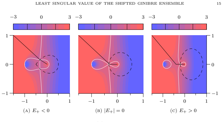
The load-bearing object is the superbosonization formula of Littelmann, Sommers and Zirnbauer, an identity that rewrites an integral over $N$ bosonic and $N$ fermionic variables as an integral over a small supermatrix with two contour variables in the complex case and three in the real case. Applied to the resolvent trace $\mathrm{E}\operatorname{Tr}(Y-w)^{-1}$, it yields the exact double-integral representation (28) for complex $X$ and the triple-integral representation (34) for real $X$, with meromorphic phase functions $f(x)=\log\frac{1+x}{x}-\frac{|z|^2}{1+x}-wx$ and $g(a,\tau,\eta)$. These representations reduce the problem to low-dimensional contour integrals whose phase is governed by the cubic equation (11) of the matrix Dyson equation; outside the critical scale $c(N,z)$ a saddle-point analysis applies, while inside it the paper rescales the integral by $|z_*|$ and extracts a universal double-integral limit. Appendix A extends the superbosonization identity from holomorphic to the meromorphic functions (26)--(27), which is the step that makes the whole representation valid.
What would settle it
For real Ginibre matrices of size $N=200$, sample $\mathrm{P}(\lambda_1(Y_z)\le c(N,z)x)$ for $z=1$ and $z=i$ at several small $x$; the theorem predicts a factor-$e^{-N/2}$ suppression of the $\sqrt{x}$ term at $z=i$ but not at $z=1$. Numerically observing the same tail exponent for the two shifts, or a violation of the bound (17) at any fixed $x$, would contradict the central claim. A more direct check is to evaluate the real-case integral (34) at $z=i$, $\delta=0$, $E=c(N)x$ and verify the claimed upper bound (15).
Extended reading notes
Core claim
The paper's central claim is that for the shifted Ginibre ensemble $Y_z=(X-z)(X-z)^*$, the least singular value $\lambda_1(Y_z)$ has, uniformly for $1-|z|^2 > -C N^{-1/2}$, the lower tail $$\mathrm{P}\big(\lambda_1(Y_z)\le c(N,z)x\big)\lesssim (1+|\log x|)\,x$$ in the complex case, and $$\mathrm{P}\big(\lambda_1(Y_z)\le c(N,z)x\big)\lesssim $e^{{-\frac12 N(\Im z)^2}}$\sqrt{x} + (1+|\log x|)\,x$$ in the real case, where $c(N,z)=\min\{N^{-3/2},\, N^{-2}|1-|z|^2|\}$. The bound is optimal up to logarithmic corrections: at $z=0$ it reproduces Edelman's exact tails, and it improves the classical uniform bound $\mathrm{P}(\lambda_1\le x N^{-2})\lesssim \sqrt{x}$ of Sankar, Spielman and Teng in precisely the transitional regime where the spectral edge sits at a distance comparable to the eigenvalue spacing. The real-case formula exhibits a transition: when $\Im z$ is of order one, the exponential factor suppresses the $\sqrt{x}$ term, so real matrices behave like complex ones, whereas near $\Im z=0$ the real $\sqrt{x}$ behavior survives.
Load-bearing premise
The argument depends on extending the superbosonization identity to the meromorphic function in (26)/(27), whose pole at $\langle s,s\rangle=iN$ is away from the integration domain; if that extension is not valid, the integral representations (28) and (34), and hence every later bound, would lose their foundation.
Editorial extensions
If this is right
- At $z=0$ the new bound matches Edelman's exact tails ($x$ in the complex case, $\sqrt{x}$ in the real case), showing that the improvement is sharp up to logarithms.
- For shifts with $1-|z|^2$ between $-C N^{-1/2}$ and $1$, the old $N^{-2}$-scale universal bound is replaced by the smaller scale $c(N,z)$, and the tail at that scale has power-law order $x$ up to logs.
- In the real case, a shift with nonzero imaginary part removes the $\sqrt{x}$ behavior, so real matrices inherit the complex tail away from the real axis.
- The paper states that this tail bound supplies the missing input used in a companion work to prove edge universality for non-Hermitian random matrices with i.i.d. entries.
- The bound also feeds into central limit theorems for linear eigenvalue statistics of complex and real i.i.d. matrices, as the paper notes.
Reading between the lines
- If the bound is right, the same optimal order should extend to smoothed-analysis condition numbers for rank-one perturbations $A_0+X$ when the determinant of $A_0$ is near the spectral edge, since the shift $z$ is the rank-one case.
- The explicit real/complex transition suggests that local edge statistics of real non-Hermitian matrices should interpolate between symmetry classes depending on $\Im z$, a phenomenon not established in the paper itself.
- One can test the predicted $e^{-N(\Im z)^2/2}$ suppression numerically by sampling real Ginibre matrices at $z=1$ and $z=i$ and comparing the tail exponents, which would give a direct check of the transition.
Signed reviews
Editorial analysis
A structured set of objections, weighed in public.
Referee Report
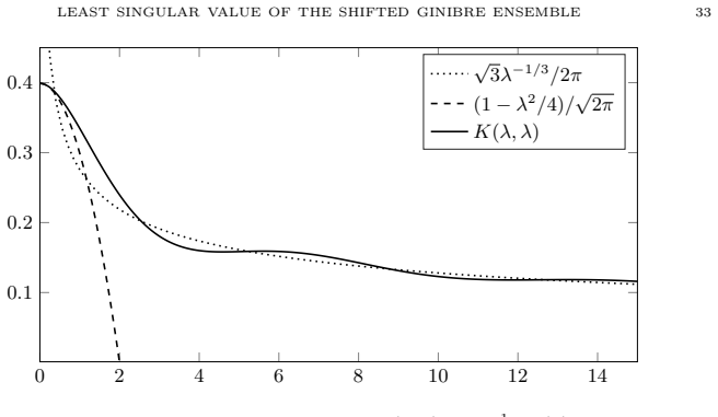
Summary. The paper studies the smallest eigenvalue λ1(Y_z) of Y_z=(X-z)(X-z)^* for N×N real or complex Ginibre matrices X, in the edge regime |z|≤1+CN^{-1/2}. The main result, Corollary 2.4, asserts the optimal lower tail bound P(λ1(Y_z)≤c(N,z)x)≲(1+|log x|)x in the complex case and P(...)≲e^{-N(Im z)^2/2}√x+(1+|log x|)x in the real case, with c(N,z)=min{N^{-3/2},N^{-2}|1-|z|^2|}. The proof uses the superbosonization formula to reduce the averaged resolvent trace to low-dimensional contour integrals: Theorem 2.1 gives an asymptotic formula in the complex case and Theorem 2.3 gives a bound on E Tr(Y+E)^{-1} in the real case; Corollary 2.4 is stated to follow by a Markov inequality. The complex-case derivation is corroborated against the Ben Arous–Péché kernel in Appendix C.
Significance. If correct, the result is a substantial improvement over the classical Sankar–Spielman–Teng bound in the previously unexplored edge regime, and it identifies a sharp real/complex transition controlled by Im z. The paper's strengths are its explicit use of the superbosonization method, the absence of fitted parameters, and the independent confirmation of the complex one-point function against the known contour-integral kernel in Appendix C. The real-case result is novel and goes beyond available Brézin–Hikami formulas.
major comments (3)
- [Theorem 2.3, Eq. (15)] The first term e^{-N(Im z)^2/2}(N^{3/4}∨N√|δ|)√E in the bound on |E Tr(Y+E)^{-1}| has the wrong E-scaling to imply the √x term in Corollary 2.4 via the stated Markov step. For E=xc(N,z), at δ=0 this term is O(√x), and after multiplying by the Markov factor 2E it becomes O(x^{3/2}N^{-3/2}), which is far smaller than √x; at δ=1 it is O(√x), and the same problem occurs. Moreover, for z=0 (δ=1), the known real Ginibre result (3) implies E Tr(XX*+xN^{-2})^{-1}∼N^2/√x for fixed small x, which contradicts the displayed √x term of (15). The lemmas in Section 6 suggest the intended first term is proportional to E^{-1/2}, not √E; if so, Eq. (15) must be corrected and the proof of Theorem 2.3 must be checked to confirm the E^{-1/2} factor.
- [Corollary 2.4] The derivation of Corollary 2.4 from Theorems 2.1 and 2.3 is not written out, and the advertised 'straightforward Markov inequality' is not straightforward in the stated form. In the complex case the needed step is an eigenvalue-counting inequality such as P(λ1≤E)≤π^{-1}∫_0^E Im E Tr(Y-t+i0)^{-1} dt, which should be stated explicitly because Theorem 2.1 bounds the trace, not the counting function. In the real case, after the correction of (15), the step P(λ1≤E)≤2E E Tr(Y+E)^{-1} should be displayed; without it, the claimed √x term has no visible proof. This omission is load-bearing because Corollary 2.4 is the main result of the paper.
- [Section 6, proof of Theorem 2.3] The proof of Theorem 2.3 in the case δ≥0 consists of a single sentence referring to Lemma 6.4 and the expansions (76)–(77). Given that the statement of (15) appears to contain a scaling error, the real-case proof needs to be expanded to show how the e^{-N(Im z)^2/2}E^{-1/2} (or corrected) term, the N^{3/2}(1+|log(NE^{2/3})|) term, and the δ<0 case are obtained from Lemmas 5.2, 6.2, 6.3 and 6.4. As written, the proof is not sufficiently checkable for a result of this specificity.
minor comments (4)
- [Theorem 2.3] The statement 'uniformly in E≥0' is incompatible with the factor 1+|log(NE^{2/3})|, which is singular at E=0; the statement should restrict to E>0 or clarify the interpretation of the logarithmic factor at E=0.
- [Appendix A] The justification of the superbosonization identity for the meromorphic function F in (26)/(27) is an outlined approximation argument. Since this is a load-bearing analytic premise, the approximation steps in Appendix A should be presented in complete detail, in particular the Laguerre-polynomial approximation for coefficient functions with a pole at −1 and the control of the truncation order in the y-integration.
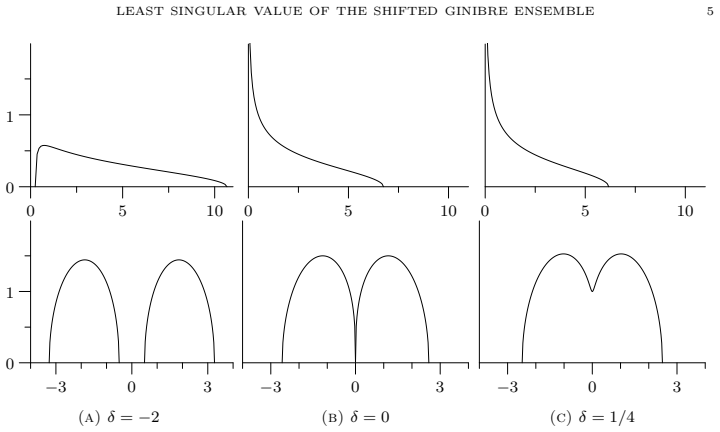
- [Figure 1] The caption of Figure 1 states that the difference between x- and √x-scaling is 'observable' for real z=±1, but it does not specify the x-axis scaling used in the second plot; this should be stated so that the reader can verify the claimed exponent against the theoretical c(N,z).
- [Introduction, Eq. (4a)] The notation ≲ in (4a) should specify that the constants are uniform in the stated x-range and in N→∞; currently the uniformity is only described in Corollary 2.4.
Circularity Check
No significant circularity: the derivation is self-contained, using the external superbosonization identity and explicit resolvent estimates, with self-citations serving only as applications.
full rationale
The paper's derivation chain is not circular. The central input, the superbosonization formula, is an externally established identity [45] (with conditions extended in Appendix A via explicit approximation arguments), not a result of the present authors. The main estimates (Theorems 2.1 and 2.3) are proved by contour deformation and saddle point analysis of the resulting integral representations (28) and (34); no parameter is fitted to the target tail probability, and the scaling factor c(N,z) is derived from the resolvent analysis rather than defined so that the tail bound becomes tautological. Corollary 2.4 is stated as a straightforward Markov consequence of the resolvent bounds; while its derivation is terse and may deserve more detail, this is a proof exposition issue, not a circular reduction, since the resolvent bounds are independent of the tail assertion. The self-citations [20,21,22] are described as applications of the present result, not as inputs to it. The acknowledgement in Appendix C that the complex-case 1-point function coincides with the known Bessel-kernel expression from [10] is a transparent statement of prior overlap, not a renaming presented as new evidence. No circular step satisfying the required standard (an equation reducing to its inputs by construction) is present.
Assumptions & free parameters
assumptions (4)
- ad hoc to paper The superbosonization identity [45] applies to the meromorphic function F in (26)/(27) after the approximation procedure in Appendix A.
- standard math The contour deformations for the x and y integrations are valid and do not cross essential singularities at 0 and -1 in the complex case, or preserve the real-case constraints in (33).
- standard math The saddle point approximation formula (42) is applicable with controlled remainder in all noncritical regimes.
- standard math The block matrix identity (8) and Gaussian integration over the Ginibre matrix X are exact.
Cite this review
Pith. "Pith review of Optimal Lower Bound on the Least Singular Value of the Shifted Ginibre Ensemble." pith.science (2026). https://pith.science/paper/4ILJ6V7T
@misc{pith2026190801653,
  author       = {Pith},
  title        = {Pith review of: Optimal Lower Bound on the Least Singular Value of the Shifted Ginibre Ensemble},
  year         = {2026},
  howpublished = {\url{https://pith.science/paper/4ILJ6V7T}},
  note         = {Machine review of arXiv:1908.01653}
}
abstract
We consider the least singular value of a large random matrix with real or complex i.i.d. Gaussian entries shifted by a constant $z\in\mathbb{C}$. We prove an optimal lower tail estimate on this singular value in the critical regime where $z$ is around the spectral edge thus improving the classical bound of [Sankar, Spielman, Teng, 2006] in the edge regime. Lacking Br\'ezin-Hikami formulas in the real case, we rely on the superbosonization formula [Littelmann, Sommers, Zirnbauer, 2008].
Figures

Figures from the paper (4 more)


Forward citations
Cited by 1 Pith paper
-
Universality of the least singular value for the sum of random matrices
The least singular value of R*XT + U*YV, after scaling by N, converges in distribution to 1 - e^{-r^2}, the same limit as for a complex Gaussian matrix.
Reference graph
Works this paper leans on
-
[1]
Spectral radius of random matrices with independent entries
1I. Afanasiev, On the correlation functions of the characteristic polynomials of non- Hermitian random matrices with independent entries , J. Stat. Phys. 176, 1561–1582 (2019), MR4001834. 2O. H. Ajanki, L. Erd˝ os, and T. Kr¨ uger, Stability of the matrix Dyson equation and random matrices with correlations, Probab. Theory Related Fields 173, 293–373 (201...
work page Pith review arXiv 2019
-
[2]
Universality of the least singular value for the sum of random matrices
Mathematics, Edited and with a foreword by A. A. Kirillov, With an appendix by V. I. Ogievetsky, Translated from the Russian by J. Niederle and R. Koteck´ y, Translation edited by Dimitri Le˘ ıtes (D. Reidel Publishing Co., Dordrecht, 1987), pp. xii+424, MR914369. 12C. Bordenave, P. Caputo, D. Chafa¨ ı, and K. Tikhomirov, On the spectral radius of a rando...
work page Pith review arXiv 2018
-
[3]
Universality for 1 d random band matrices
Press, New York-London, 1967), pp. x+259, MR0220494. 48M. Y. Mo, Rank 1 real Wishart spiked model , Comm. Pure Appl. Math. 65, 1528–1638 (2012), MR2969495. 49J. Osborn, D. Toublan, and J. Verbaarschot,From chiral random matrix theory to chiral perturbation theory, Nuclear Physics B 540, 317–344 (1999). 50C. Recher, M. Kieburg, T. Guhr, and M. Zirnbauer,Su...
work page Pith review arXiv 2012
Reviewed August 14, 2026 · model on record in the stance chip above.
Discussion (0). Continue with ORCID to comment.