pith. sign in

arxiv: 2605.28596 · v1 · pith:4KY7BYOInew · submitted 2026-05-27 · 🌌 astro-ph.CO · cs.LG

Dark Quest II: A Wide-Coverage Neural Network Emulator of the Nonlinear Matter Power Spectrum Across Extended Cosmologies

Pith reviewed 2026-06-29 10:46 UTC · model grok-4.3

classification 🌌 astro-ph.CO cs.LG
keywords cosmological emulatormatter power spectrumneural networkN-body simulationsdark energyneutrino massnonlinear structure
0
0 comments X

The pith

Neural network emulator matches nonlinear matter power spectra to subpercent accuracy up to the Nyquist scale across nine-dimensional cosmologies.

A machine-rendered reading of the paper's core claim, the machinery that carries it, and where it could break.

The paper introduces DarkEmulator2, a neural network that emulates the nonlinear matter power spectrum over a nine-dimensional parameter space that includes w0, wa, neutrino mass, and other cosmological parameters. It trains on N-body simulations from the Dark Quest II program, supplementing the network inputs with the linear power spectrum, simulation resolution descriptors, and a summary of the initial Gaussian random field. The network is trained jointly across three resolution tiers to combine broad coverage from lower-resolution runs with precision from a smaller set of high-resolution runs. For a 1 Gpc box with 3000 cubed particles, this yields subpercent accuracy up to k approximately 10 h per Mpc, with validation against independent tests and comparisons to other emulators.

Core claim

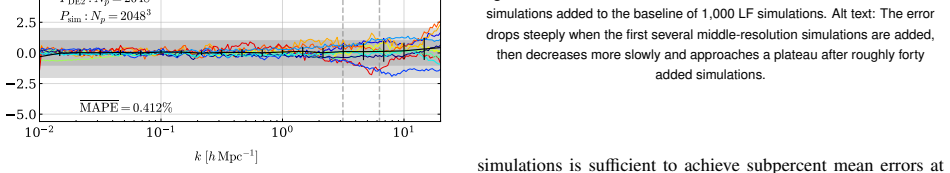
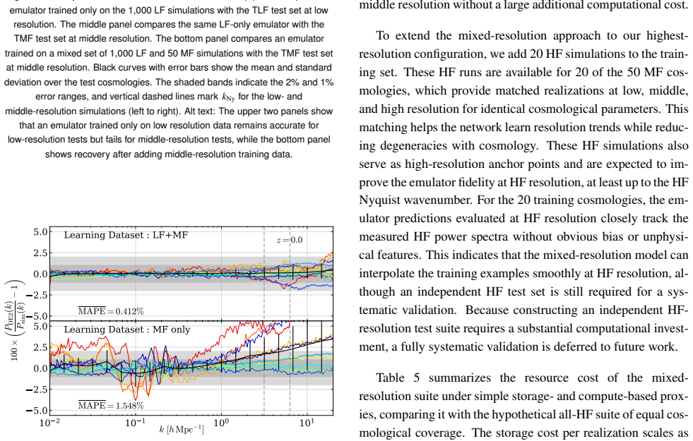
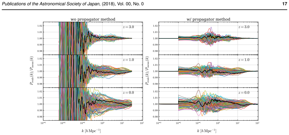
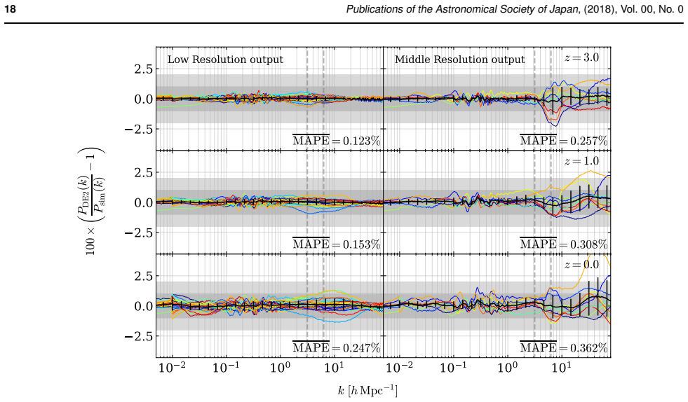
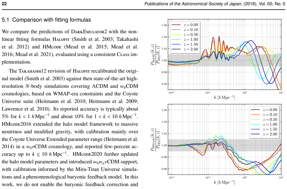
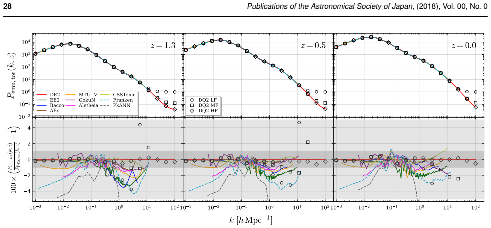
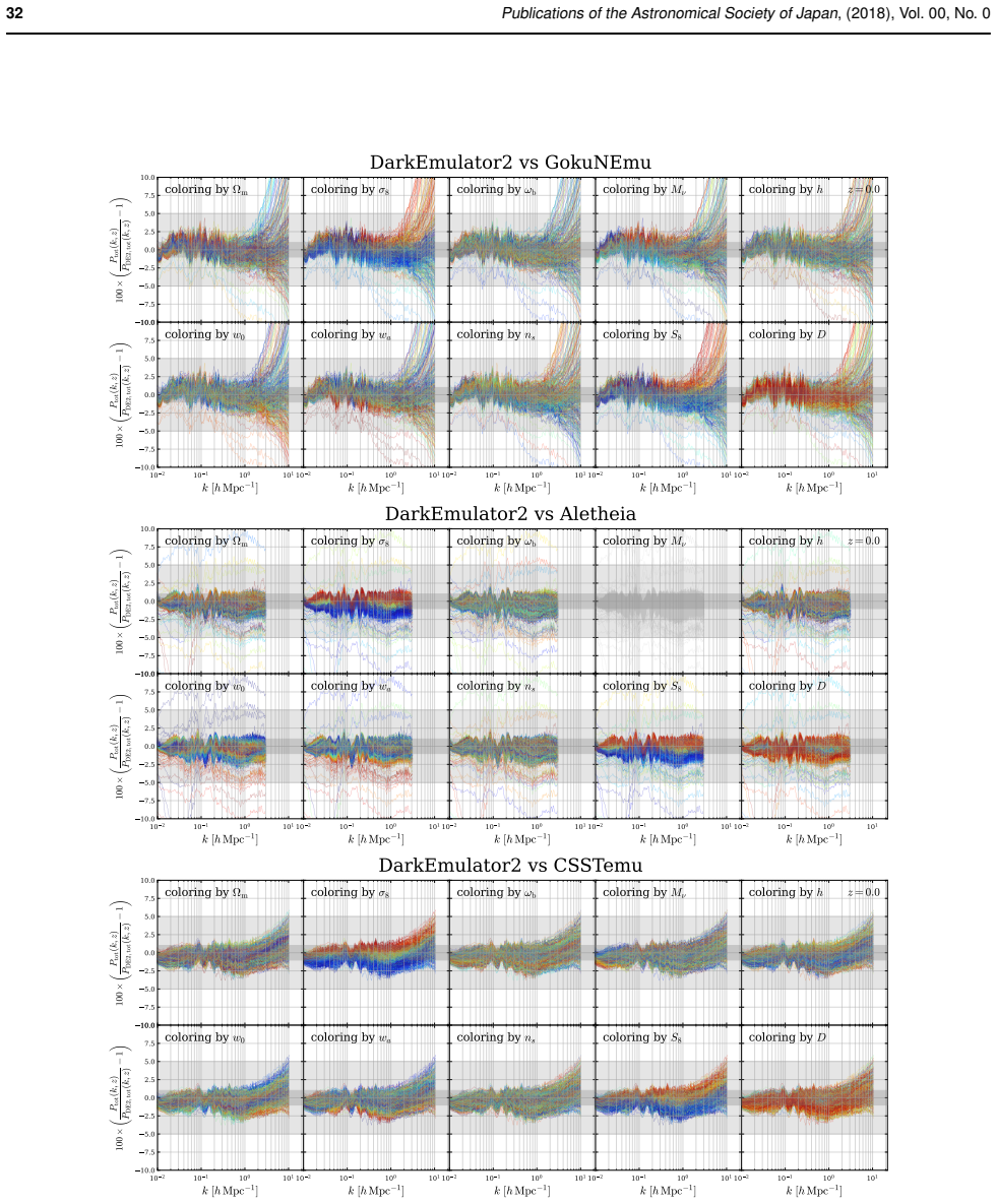
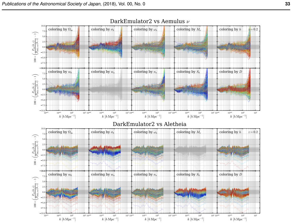
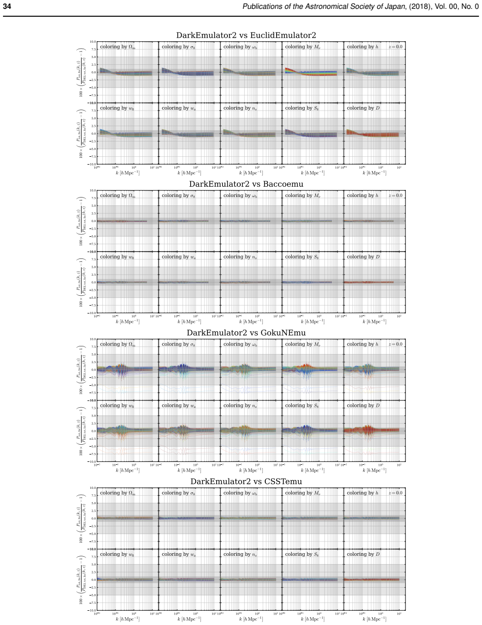
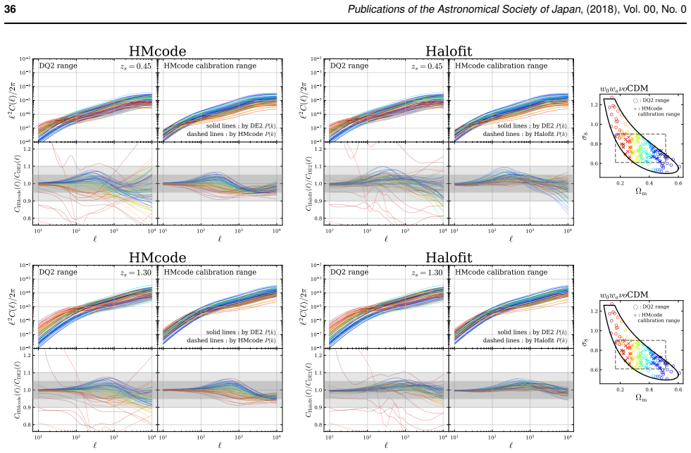
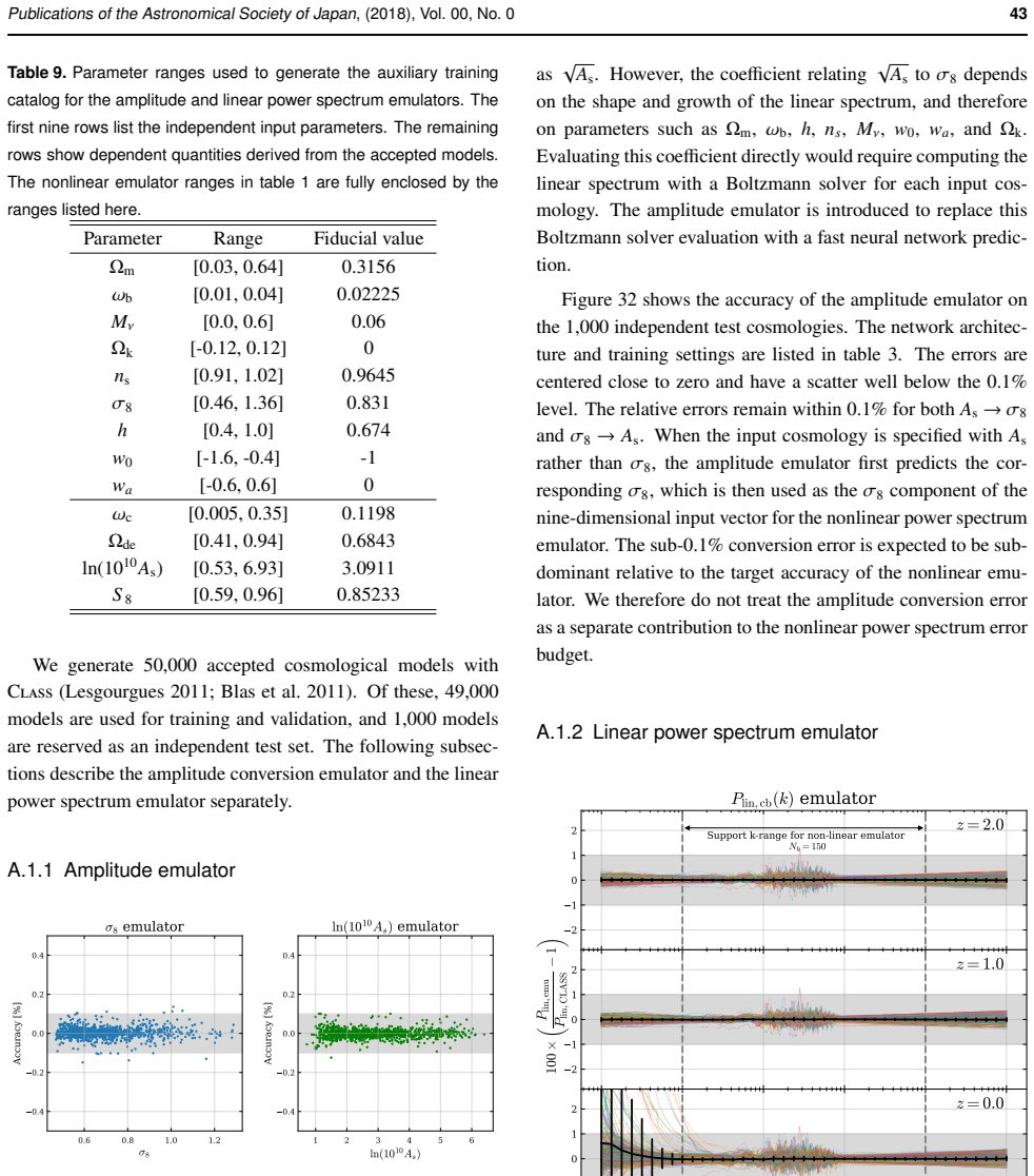
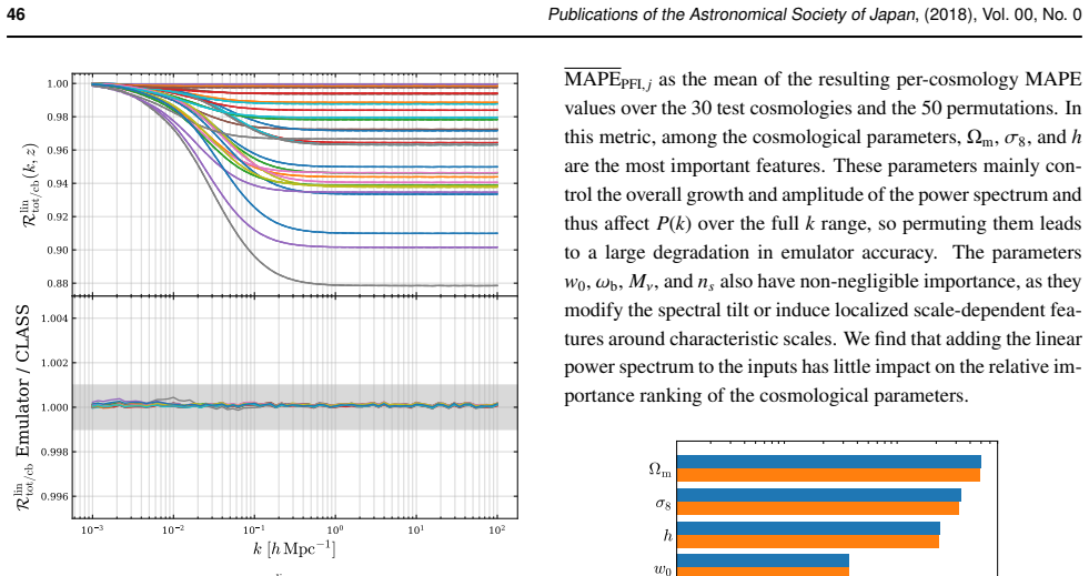
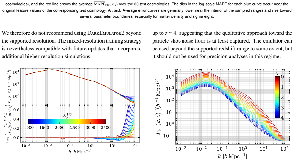
DarkEmulator2 reproduces the simulated matter power spectrum to subpercent accuracy up to the particle Nyquist scale k_Ny ≃ 10 h/Mpc for a 1 Gpc box with 3000^3 particles, remaining accurate over the calibrated wavenumber range while its highest-k predictions depend on simulation resolution and shot noise.

What carries the argument

A single neural network trained jointly across three simulation resolution tiers, taking as inputs the cosmological parameter vector supplemented by the linear matter power spectrum, descriptors of simulation resolution, and a low-dimensional summary of the initial Gaussian random field.

Load-bearing premise

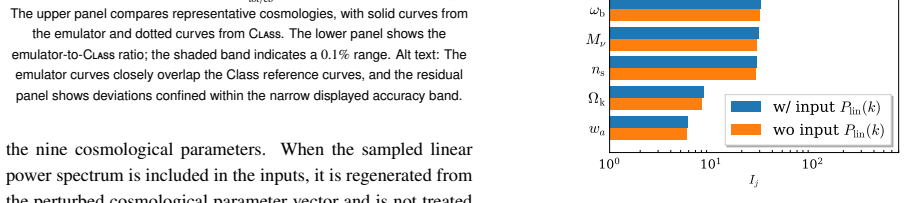
Supplementing the neural network inputs with the linear matter power spectrum, descriptors of simulation resolution, and a low-dimensional summary of the initial Gaussian random field will improve generalization across the nine-dimensional parameter space.

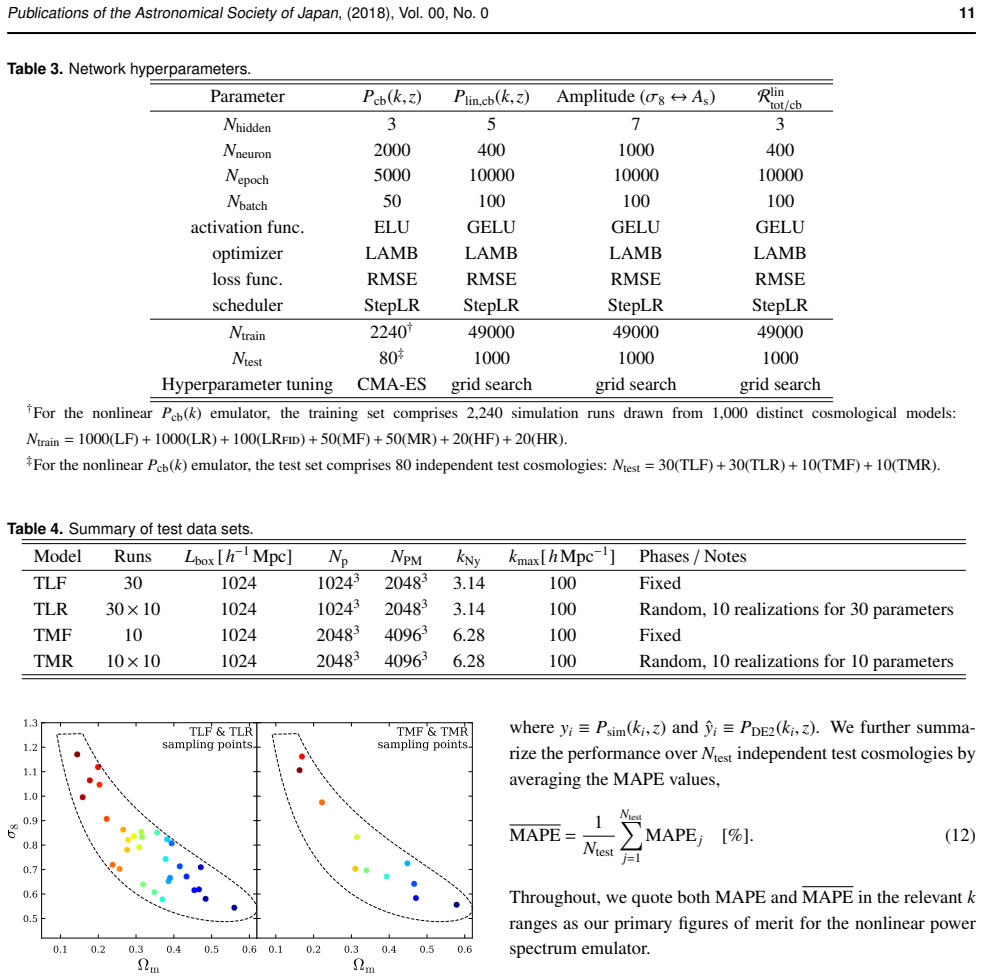
What would settle it

Running the emulator on a new independent suite of high-resolution simulations spanning the same nine-dimensional space and checking whether subpercent agreement holds up to k_Ny ≃ 10 h/Mpc.

Figures

Figures reproduced from arXiv: 2605.28596 by Satoshi Tanaka, Takahiro Nishimichi, Yosuke Kobayashi.

Figure 1
Figure 1. Figure 1: Distribution of 1,000 cosmologies in the nine-dimensional parameter space. Colors encode Ωm; the star marks the fiducial model. The independent set is (Ωm,ωb,σ8,ns ,h, Mν,w0,wa,Ωk); dependent quantities (ωc,Ωde,S 8) are shown for reference. Alt text: Corner plot with one-dimensional parameter distributions on the diagonal and pairwise projections off the diagonal. 0.1 0.3 0.5 ­m 0 1 2 3 4 5 D 0.1 0.2 !c 0.… view at source ↗
Figure 2
Figure 2. Figure 2: Same sample as figure 1, colored by the linear spectrum distance D defined in equation 2. Alt text: Row of scatter panels comparing the distance metric with individual cosmological parameters. The strongest visible trends occur for matter density, cold dark matter density, and sigma eight [PITH_FULL_IMAGE:figures/full_fig_p006_2.png] view at source ↗
Figure 3
Figure 3. Figure 3: Random samples of training targets across cosmologies, redshifts, and resolutions. Colors encode the linear power spectrum distance D (blue: small, red: large). The top, second, third, and bottom panels show the original nonlinear “cb” power spectrum Psim(k,z), the nonlinear boost factor Bfid(k,z), the log-ratio Y(k,z), and the tapered target Y˜(k,z), respectively. Alt text: Four stacked line plots in whic… view at source ↗
Figure 4
Figure 4. Figure 4: Overview of the DarkEmulator2 emulator architecture. Alt text: Flowchart showing connected emulator modules that combine cosmological inputs, redshift, resolution information, and optional white noise variables to produce matter power spectra. for validation. The 10% subset in each MCCV split is a vali￾dation set used during training and should not be confused with the independent test suite described belo… view at source ↗
Figure 5
Figure 5. Figure 5: Distribution of test cosmologies in the Ωm-σ8 plane. The left panel shows the low-resolution test sets (TLF/TLR) and the right panel shows the middle-resolution test sets (TMF/TMR). The color coding, with red indicating smaller Ωm and blue larger Ωm, is reused in the figures comparing emulator predictions to these test sets. Alt text: Points lie within a dashed, banana-shaped support region and follow a de… view at source ↗
Figure 6
Figure 6. Figure 6: Accuracy of the emulator trained on the 1,000 LF cosmologies, evaluated on the 30 test cosmologies. The left panels use only the nine-dimensional cosmological parameter vector as input, whereas the right panels additionally include the linear power spectrum as input features. For k < 0.01 hMpc−1 , the residual is evaluated against the linear-theory spectrum predicted by the linear emulator, whereas for k ≥… view at source ↗
Figure 7
Figure 7. Figure 7: Ratios of the LF (red) and MF (blue) matter power spectra to the corresponding HF results. Each curve corresponds to one of the 20 cosmological models with matched LF, MF, and HF simulations. Vertical dashed lines mark kNy for the LF, MF, and HF simulations (left to right). Alt text: Lower-resolution spectra depart from the high-resolution reference before their Nyquist scales, with larger departures at hi… view at source ↗
Figure 10
Figure 10. Figure 10: MAPE on the TMF test set at z = 0 as a function of the number of MF simulations added to the baseline of 1,000 LF simulations. Alt text: The error drops steeply when the first several middle-resolution simulations are added, then decreases more slowly and approaches a plateau after roughly forty added simulations. simulations is sufficient to achieve subpercent mean errors at middle resolution without a l… view at source ↗
Figure 8
Figure 8. Figure 8: Accuracy of the mixed-resolution emulator. The top panel compares an emulator trained only on the 1,000 LF simulations with the TLF test set at low resolution. The middle panel compares the same LF-only emulator with the TMF test set at middle resolution. The bottom panel compares an emulator trained on a mixed set of 1,000 LF and 50 MF simulations with the TMF test set at middle resolution. Black curves w… view at source ↗
Figure 9
Figure 9. Figure 9: Accuracy on the TMF test set. The upper panel shows the emulator trained on 1,000 LF + 50 MF models, and the lower panel shows the emulator trained on 50 MF models only. Plotting conventions are the same as in figure 8. Alt text: The mixed low- and middle-resolution training set gives residuals clustered near zero, whereas the model trained only on middle resolution data shows larger scatter and systematic… view at source ↗
Figure 11
Figure 11. Figure 11: Ratio of the nonlinear total matter power spectrum of each realization to the mean over 100 realizations of the fiducial cosmology in the low-resolution model LRfid. The left panel shows the ratios without the propagator method, and the right panel shows the ratios after applying the propagator method of Nishimichi et al. (2026). The black curves highlight the realizations corresponding to the fixed-phase… view at source ↗
Figure 12
Figure 12. Figure 12: illustrates the behavior of our white noise genera￾tor based on these statistics. For each k-bin, we draw 1,000 re￾alizations of W(k) with the appropriate k-dependent number of nk. The black line with error bars shows the mean and standard deviation over the 1,000 realizations, while the green dashed lines indicate the analytic expectation from the χ 2 distribution. These results confirm that the generato… view at source ↗
Figure 13
Figure 13. Figure 13: Conditional consistency test of the cosmic-variance-aware emulator when random-phase models are included in the training data. The left panels show results for the low-resolution training configuration (LF+LR+LRfid), and the right panels additionally include middle-resolution models (+MF+MR). For each test cosmology, we compare the mean of 10 N-body realizations to the mean of 10 emulator outputs evaluate… view at source ↗
Figure 14
Figure 14. Figure 14: Realization-level response of the white-noise-conditioned emulator at z = 0. The upper and lower rows show 20 selected curves from the low- and middle-resolution random-phase test sets, respectively, spanning different cosmological parameters and initial-condition white-noise patterns. Within each row, the panels show the simulation response, the emulator response with the same white-noise inputs, and the… view at source ↗
Figure 15
Figure 15. Figure 15: Comparison between the ensemble average obtained by explicitly averaging over white noise realizations and the single emulator evaluation at the all-ones white noise input. The left panel shows the fractional difference between the average over 500 emulator evaluations with independent white noise inputs, ⟨Pemu(k,z,θ,W)⟩W, and the emulator prediction evaluated once with the white noise vector set to unity… view at source ↗
Figure 16
Figure 16. Figure 16: Validation of the calibrated fast ensemble-mean prediction for the fiducial cosmology of the low-resolution model LRfid. All curves are shown as ratios to the simulation mean P rand100 sim,fid (k), minus unity. Thin gray curves show the 100 individual simulation realizations P (r) sim,fid(k). The red curve shows P rand100 emu,fid (k), computed with the same white-noise inputs as the simulations. The cyan … view at source ↗
Figure 17
Figure 17. Figure 17: compares the nonlinear total matter power spec￾trum Ptot(k) predicted by DarkEmulator2 with the fitting for￾mulas at the DQ2 fiducial cosmology. For both Halofit and HMcode, the discrepancies are typically within about 5% for k < 1 h Mpc−1 and increase to about 10% at lower redshift once k > 1 h Mpc−1 . Similar residual patterns were also re￾ported by Euclid Collaboration et al. (2021). Around the BAO ran… view at source ↗
Figure 18
Figure 18. Figure 18: Comparison of DarkEmulator2 with nonlinear fitting formulas for 80 randomly sampled cosmologies. The upper block shows ΛCDM models, and the lower block shows extended dark energy models. In each block, the left large panel shows HMcode, and the middle large panel shows Halofit. Within each large panel, the upper row corresponds to z = 1 and the lower row to z = 0; the left subcolumn uses cosmologies sampl… view at source ↗
Figure 19
Figure 19. Figure 19: Parameter ranges on the Ωm-σ8 plane for this work and other public emulators. For several emulators that do not explicitly include Ωm or σ8 as input parameters, we derive these quantities from their native cosmological parameters. The star symbol indicates the Planck 2015 best-fit cosmology and the fiducial cosmology of DQ2. Alt text: Support regions of public emulators mostly occupy narrower central part… view at source ↗
Figure 20
Figure 20. Figure 20: Parameter, wavenumber, and redshift ranges for DarkEmulator2 and other public nonlinear matter power spectrum emulators considered in this work. For each parameter, horizontal segments show the support range covered by each emulator. Solid lines denote the ranges of the native input parameters used in the design of each emulator. Dashed lines indicate the ranges of derived parameters inferred from over 1,… view at source ↗
Figure 21
Figure 21. Figure 21: Comparison of the total matter power spectra at the DQ2 fiducial cosmology. The top panels show Ptot(k) from each emulator, and the bottom panels show the ratios relative to DarkEmulator2. From left to right, the redshift is z = 1.3, 0.5, and 0.0. Light and dark shaded regions indicate ±5% and ±1% deviations, respectively. Symbols show N-body simulation results for the LF, MF, and HF models with fixed-pha… view at source ↗
Figure 22
Figure 22. Figure 22: Ratios of the nonlinear total matter power spectra predicted by EuclidEmulator2 (top) and BaccoEmu (bottom) to the DarkEmulator2 prediction for 500 cosmologies randomly sampled from the parameter volume jointly supported by DarkEmulator2 and the corresponding emulator in the w0waνCDM cosmology at z = 0. Each panel shows the same set of ratio curves, but the curves are re-colored in each panel according to… view at source ↗
Figure 23
Figure 23. Figure 23: Same as figure 22, but for comparisons with Mira-Titan Univ. IV (top) and Aemulusν (bottom). Only Aemulusν employs the w0νCDM cosmology. Panels that are gray are parameters that are not in this comparison. Alt text: Mira-Titan shows broad scale-dependent suppression relative to DarkEmulator2, while Aemulus nu is mostly closer except for excursions at low wavenumber in a subset of edge cosmologies. already… view at source ↗
Figure 24
Figure 24. Figure 24: figure 24. Clear color gradients are visible in the [PITH_FULL_IMAGE:figures/full_fig_p031_24.png] view at source ↗
Figure 24
Figure 24. Figure 24: Same as figure 22, but for comparisons with GokuNEmu (top), Aletheia (middle), and CsstEmulator (bottom). For GokuNEmu, the additional parameters Neff and αs are held fixed to their default values in this comparison. Aletheia does not support massive neutrinos, and we therefore restrict the comparison to Mν = 0 and the curvature is also held fixed to Ωk = 0. Panels that are gray are parameters that are no… view at source ↗
Figure 25
Figure 25. Figure 25: Same as Figures 23 and 24, but showing the comparison between DarkEmulator2 and Aemulusν or Aletheia at z = 0.2. Alt text: At redshift 0.2, the strongest excursions at low wavenumber seen for Aemulus nu are reduced, whereas some Aletheia outliers remain visible across the plotted range. is computed with CLASS. Accordingly, the “linear” curves shown for EuclidEmulator2 in figure 26 reflect the Class pre￾di… view at source ↗
Figure 26
Figure 26. Figure 26: Same as figure 22, but for the linear total matter power spectrum Ptot,lin(k) at z = 0. In addition to nonlinear spectra, EuclidEmulator2, BaccoEmu, GokuNEmu, and CsstEmulator provide Ptot,lin(k) through their public interfaces. For BaccoEmu, GokuNEmu, and CsstEmulator, the linear spectra are produced by their internal emulators, whereas EuclidEmulator2 returns a Class-computed Ptot,lin(k) that is used to… view at source ↗
Figure 27
Figure 27. Figure 27: Comparison of C(ℓ) predicted from nonlinear P(k) by DarkEmulator2 with HMcode and Halofit in w0waνoCDM for 80 randomly sampled cosmologies. The top panels show zs = 0.45, and the bottom panels show zs = 1.3. For each zs , the left block compares with HMcode, and the right block compares with Halofit. Within each block, the left panel uses samples within the DarkEmulator2 support (DQ2 range), and the right… view at source ↗
Figure 28
Figure 28. Figure 28: Comparison of C(ℓ) derived from nonlinear P(k) for DarkEmulator2 and public emulators. We consider eight emulators in total, namely DarkEmulator2 and the seven public emulators shown. The left panels use 80 cosmologies sampled from the common overlap of all emulator parameter ranges with Mν = 0, wa = 0 and Ωk = 0. The right panels use 80 cosmologies sampled from the overlap between DarkEmulator2 and each … view at source ↗
Figure 29
Figure 29. Figure 29: Response of the nonlinear total matter power spectrum to one-parameter variations around the fiducial cosmology at z = 0. The upper row shows Ptot(k,z = 0), and the lower row shows ratios to the fiducial prediction. Panels (a)–(d) vary Mν, w0, wa, and Ωk, respectively, with 40 sampled values for each parameter. Alt text: One-parameter variations change the amplitude and scale dependence of the nonlinear m… view at source ↗
Figure 30
Figure 30. Figure 30: Same as figure 29, but for the convergence power spectrum computed with a single source plane at zs = 1. The upper row shows ℓ 2Cℓ/2π, and the lower row shows Cℓ/C fid ℓ . Alt text: The same parameter variations produce smooth changes in the convergence power spectrum after line-of-sight projection [PITH_FULL_IMAGE:figures/full_fig_p038_30.png] view at source ↗
Figure 31
Figure 31. Figure 31: Clustering predictions for the DESI-based benchmark cosmologies listed in table 7. The left panel shows the nonlinear total matter power spectrum at z = 0, and the right panel shows the convergence power spectrum computed with a single source plane at zs = 1. In each panel, the upper panels show the absolute prediction and the lower panels show the ratio to the fiducial DarkEmulator2 cosmology. Alt text: … view at source ↗
Figure 32
Figure 32. Figure 32: Accuracy of the amplitude emulator on 1,000 independent test cosmologies. The left panel shows the fractional error in the recovered σ8 for inputs specified by As . The right panel shows the fractional error in the recovered ln(1010As) for inputs specified by σ8. The shaded band indicates a 0.1% error range. Alt text: Residuals for both amplitude conversions are tightly clustered within the displayed accu… view at source ↗
Figure 34
Figure 34. Figure 34: illustrates this behavior with a one-parameter se￾quence in which w0 is varied while all other cosmological pa￾rameters are held fixed at the fiducial values. This figure is in￾tended as a diagnostic of the low-k boundary case, not as a rep￾resentative example of the typical linear emulator accuracy over the training domain. To localize the low-k degradation in parameter space, fig￾ure 35 shows two-dimens… view at source ↗
Figure 35
Figure 35. Figure 35: Two-dimensional accuracy of the linear power spectrum emulator in the w0waνoCDM model. The left and right panels show the Ωm–σ8 and Ωm–w0 planes, respectively. Accuracy is quantified as the mean absolute percentage error relative to Class. Larger errors appear in the strongly negative-w0 and low-Ωm region and near parts of the boundary of the support region, including the high-σ8 side. The black dashed li… view at source ↗
Figure 36
Figure 36. Figure 36: Two-dimensional accuracy of the linear power spectrum emulator for ΛCDM cosmologies projected onto the Ωm–σ8 plane. The sampled region is motivated by the HSC-Y3 cosmic shear parameter priors of Terasawa et al. (2025) and restricted to the banana-shaped support used by the nonlinear emulator, which was designed to cover the HSC-Y1-motivated Ωm–σ8 posterior region. Alt text: The accuracy map is broadly uni… view at source ↗
Figure 37
Figure 37. Figure 37: Linear theory total-to-cb ratio R lin tot/cb(k,z) used to convert Pcb to Ptot. The upper panel compares representative cosmologies, with solid curves from the emulator and dotted curves from Class. The lower panel shows the emulator-to-Class ratio; the shaded band indicates a 0.1% range. Alt text: The emulator curves closely overlap the Class reference curves, and the residual panel shows deviations confi… view at source ↗
Figure 38
Figure 38. Figure 38: shows the permutation importance of the nine cos￾mological parameters, evaluated both without and with the sam￾pled linear power spectrum included in the inputs. We estimate the importance using the matter power spectrum in the range 0.001 < k < 10 h Mpc−1 at z = 0, using 50 independent ran￾dom permutations of feature j across the test set, and computing MAPEPFI, j as the mean of the resulting per-cosmolo… view at source ↗
Figure 39
Figure 39. Figure 39: Grouped permutation feature importance for all pairs of input cosmological parameters. The grouped importance is defined in equation A5, and the plotted color scale shows log10 Ii j. Alt text: Cells with large importance cluster around pairs containing the individually important parameters. No pair made only of weak individual parameters becomes dominant. A.3.2 Partial dependence Partial dependence (PD; H… view at source ↗
Figure 40
Figure 40. Figure 40: One-dimensional partial dependence plots for each input parameter at z = 0. The blue lines in each panel show MAPEPD,n(a; j) for individual instances (test cosmologies), and the red line shows the average MAPEPD(a; j) over the 30 test cosmologies. The dips in the log-scale MAPE for each blue curve occur near the original feature values of the corresponding test cosmology. Alt text: Average error curves ar… view at source ↗
Figure 41
Figure 41. Figure 41: Resolution extrapolation of DarkEmulator2 at the DQ2 fiducial cosmology. Curves are shown for N 1/3 p = 1500–3500 in steps of 100. Solid segments indicate the supported range, and dotted segments show extrapolation. The bottom panel shows ratios relative to the N 1/3 p = 3000 prediction. Alt text: Predictions remain smooth near the supported resolution but develop oscillatory artifacts at high wavenumber … view at source ↗
Figure 43
Figure 43. Figure 43: Shot-noise plateau suppression and high-k extension at the DQ2 fiducial cosmology. Solid curves show the emulator output for k ≤ 100 hMpc−1 . Dashed curves show slope transition determined by the slope method. Dash-dotted curves show transition at P(k) = 10Psn. Vertical lines mark the Nyquist wavenumbers for the low-, mid-, and high-resolution settings, and horizontal lines mark the corresponding shot-noi… view at source ↗
Figure 44
Figure 44. Figure 44: Demonstration of CMA-ES with σ = 0.4, λ = 36, and µ = 18. The left panel shows the 1σ contour of the multivariate normal sampling distribution over successive generations. Contours are colored by generation, and the plot shows up to 32 generations. The right panel shows the 1σ, 2σ, and 3σ contours together with the sampling points from one representative generation. Red points receive positive recombinati… view at source ↗
read the original abstract

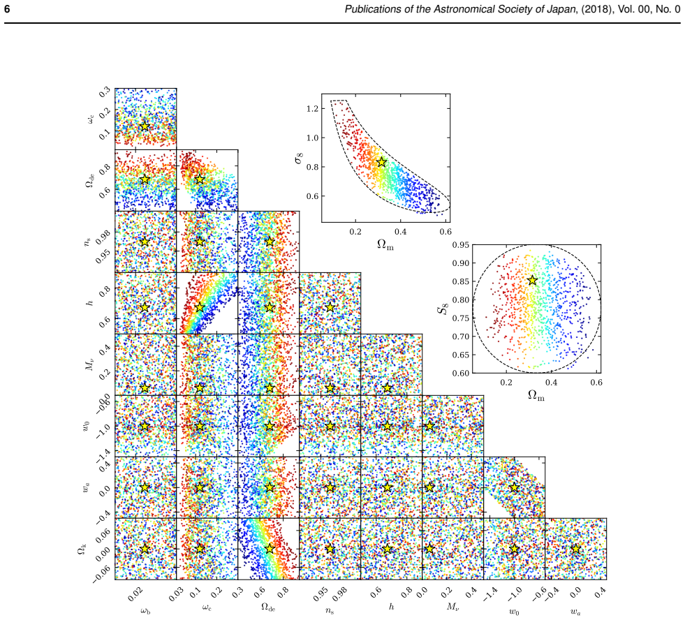
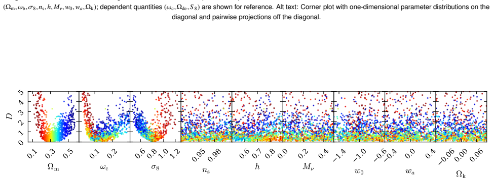
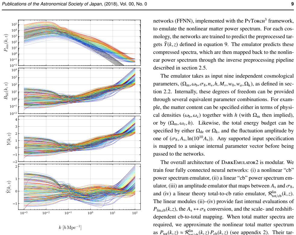
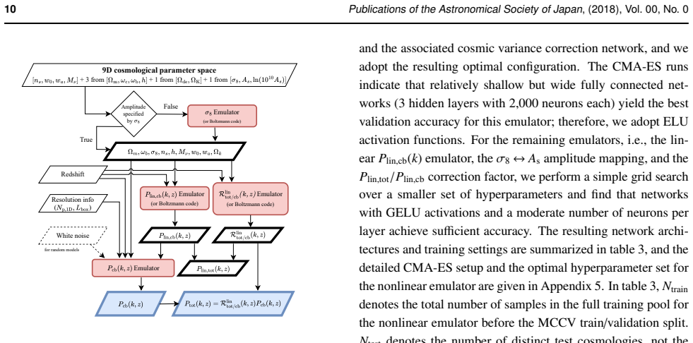
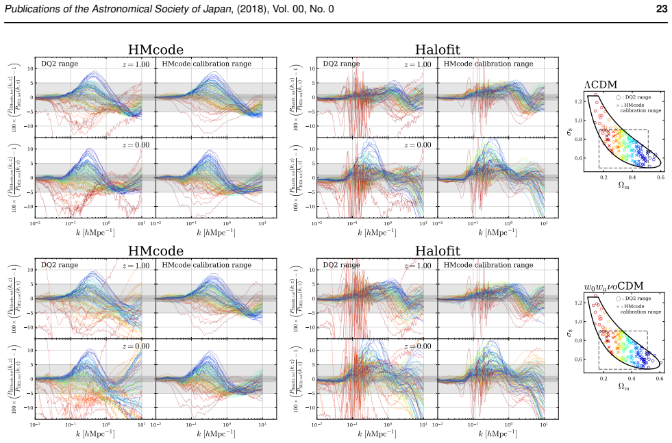
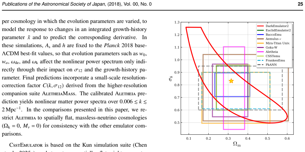
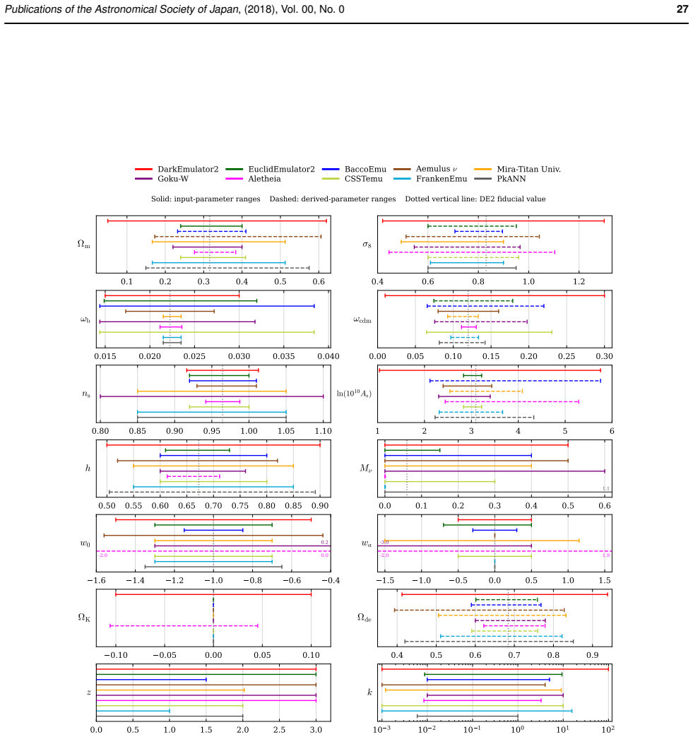
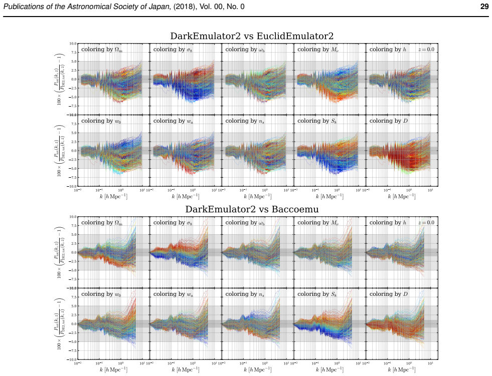
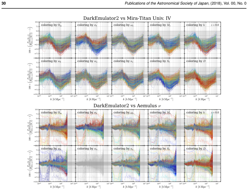
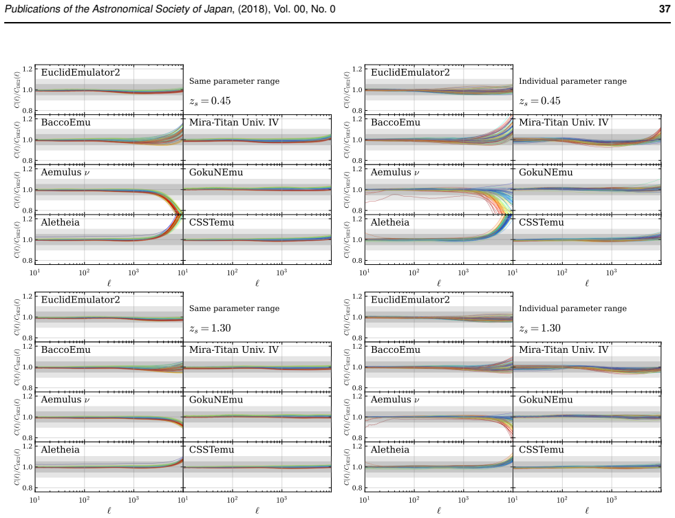
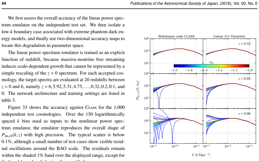
\textsc{DarkEmulator2} is a neural network emulator of the nonlinear matter power spectrum in a nine-dimensional $w_0 w_a \nu o \mathrm{CDM}$ parameter space, developed as the emulator component of the \textsc{Dark Quest II} (DQ2) program. It is trained on simulations generated with the \textsc{Ginkaku} code, whose numerical implementation, accuracy tests, and post-processing pipeline are described in the companion paper. The design follows a unified strategy: in addition to the cosmological parameter vector, we supplement the neural network's inputs with three families of physically motivated auxiliary quantities -- the linear matter power spectrum, descriptors of the simulation resolution, and a low-dimensional summary of the initial Gaussian random field -- that are expected to improve generalization across the parameter space. Training a single network jointly across three simulation resolution tiers allows the emulator to exploit a small number of high-resolution simulations while retaining broad coverage from lower-resolution simulations. For a $L_{\mathrm{box}}=1\,\hiGpc$ box with $N=3000^{3}$ particles, the emulator reproduces the simulated matter power spectrum to subpercent accuracy up to the particle Nyquist scale, $k_{\mathrm{Ny}}\simeq 10\,\hMpci$. The emulator remains accurate over the calibrated wavenumber range, while its highest-$k$ predictions depend on the simulation resolution and shot noise. We validate the emulator on independent test suites and, through a cross-comparison with several public emulators and widely used fitting formulas, characterize the inter-model consistency and the parameter-dependent trends in their residuals.

Editorial analysis

A structured set of objections, weighed in public.

Desk editor's note, referee report, simulated authors' rebuttal, and a circularity audit. Tearing a paper down is the easy half of reading it; the pith above is the substance, this is the friction.

Referee Report

2 major / 0 minor

Summary. The manuscript presents DarkEmulator2, a neural network emulator for the nonlinear matter power spectrum in a nine-dimensional w0 wa ν o CDM parameter space. It is trained jointly across three simulation resolution tiers from the Ginkaku code, with the cosmological parameter vector supplemented by the linear matter power spectrum, resolution descriptors, and a low-dimensional summary of the initial Gaussian random field. The central claim is that this single network achieves subpercent accuracy in reproducing the simulated P(k) up to the particle Nyquist scale k_Ny ≃ 10 h/Mpc for L_box=1 Gpc, N=3000^3 runs, remains accurate over the calibrated range, and is validated on independent test suites with comparisons to other emulators.

Significance. If the accuracy and generalization claims hold, the emulator would enable efficient cosmological analyses over extended parameter spaces by leveraging sparse high-resolution simulations together with broad low-resolution coverage. The joint-training strategy across resolution tiers and the use of physically motivated auxiliary inputs represent a practical approach to wide-coverage emulation; the validation on independent suites and cross-comparison with public emulators are explicit strengths that support reproducibility and inter-model assessment.

major comments (2)
  1. [Abstract] Abstract: the claim that the auxiliary inputs (linear P(k), resolution descriptors, and initial-field summary) 'are expected to improve generalization across the parameter space' is presented without ablation studies, controlled comparisons, or quantitative evidence isolating their contribution to the reported accuracy. This assumption is load-bearing for the joint-training strategy, as the ability to exploit a small number of high-resolution runs while retaining broad coverage from lower-resolution simulations rests on it.
  2. [Abstract] Abstract: the headline accuracy statement ('reproduces the simulated matter power spectrum to subpercent accuracy up to k_Ny ≃ 10 h/Mpc') supplies no quantitative error metrics (e.g., mean or maximum relative error as a function of k, cosmology, or resolution tier), details on post-hoc choices, or explicit validation statistics on the independent test suites. Without these, the central performance claim cannot be assessed for load-bearing consistency with the joint-training design.

Simulated Author's Rebuttal

2 responses · 0 unresolved

We thank the referee for their careful review and constructive feedback. We address each major comment below, indicating where revisions will be made to strengthen the manuscript.

read point-by-point responses
  1. Referee: [Abstract] the claim that the auxiliary inputs (linear P(k), resolution descriptors, and initial-field summary) 'are expected to improve generalization across the parameter space' is presented without ablation studies, controlled comparisons, or quantitative evidence isolating their contribution to the reported accuracy. This assumption is load-bearing for the joint-training strategy.

    Authors: The auxiliary inputs are motivated by physical considerations (linear power spectrum captures large-scale modes, resolution descriptors account for numerical effects, and initial-field summary encodes phase information), as detailed in the methods. The joint-training performance across tiers provides supporting evidence for their utility in generalization. We did not conduct explicit ablation studies. In revision, we will update the abstract to clarify that these inputs are included to support generalization and add a brief discussion of the training results as indirect evidence. revision: yes

  2. Referee: [Abstract] the headline accuracy statement ('reproduces the simulated matter power spectrum to subpercent accuracy up to k_Ny ≃ 10 h/Mpc') supplies no quantitative error metrics (e.g., mean or maximum relative error as a function of k, cosmology, or resolution tier), details on post-hoc choices, or explicit validation statistics on the independent test suites.

    Authors: The abstract is a concise overview; full quantitative metrics (mean/max relative errors vs. k, cosmology, and tier), validation statistics on independent suites, and cross-comparisons appear in Sections 4–5 and associated figures/tables. To address the concern, we will revise the abstract to include a brief quantitative qualifier (e.g., typical mean relative error <1% up to k_Ny on test sets) with explicit references to the detailed results. revision: yes

Circularity Check

0 steps flagged

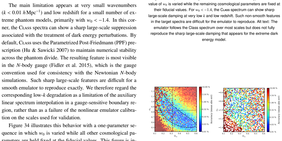
No significant circularity; emulator trained on external simulations with independent validation

full rationale

The paper trains a neural network on simulations generated by the external Ginkaku code and validates accuracy on independent test suites. Auxiliary inputs (linear P(k), resolution descriptors, initial field summary) are described as physically motivated quantities expected to aid generalization; this is an empirical design choice, not a self-definition or fitted input renamed as prediction. The sub-percent accuracy claim is a direct reproduction metric against held-out simulation data, not a quantity derived from itself by construction. No load-bearing self-citations, uniqueness theorems, or ansatzes imported from prior author work appear in the provided text. The derivation chain remains self-contained against external simulation benchmarks.

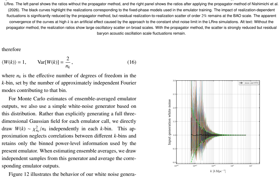
Axiom & Free-Parameter Ledger

0 free parameters · 0 axioms · 0 invented entities

Based solely on the abstract; no explicit free parameters, axioms, or invented entities are identifiable. The neural network weights constitute implicit fitted parameters standard to the method.

pith-pipeline@v0.9.1-grok · 5835 in / 1055 out tokens · 46406 ms · 2026-06-29T10:46:37.588787+00:00 · methodology

discussion (0)

Sign in with ORCID, Apple, or X to comment. Anyone can read and Pith papers without signing in.

Reference graph

Works this paper leans on

128 extracted references · 3 canonical work pages · 2 internal anchors

  1. [1]

    B., Aleksi ´c, J., et al

    Abbott, T., Abdalla, F. B., Aleksi ´c, J., et al. 2016, Mon. Not. R. Astron. Soc., 460, 1270

  2. [2]

    Abbott, T. M. C., Aguena, M., Alarcon, A., et al. 2022, Phys. Rev. D, 105, 023520 Abdul Karim, M., Aguilar, J., Ahlen, S., et al. 2025, Phys. Rev. D., 112, 083515 Publications of the Astronomical Society of Japan , (2018), Vol. 00, No. 0 51

  3. [3]

    B., Feldman, H

    Agarwal, S., Abdalla, F. B., Feldman, H. A., Lahav, O., & Thomas, S. A. 2012, MNRAS, 424, 1409 —. 2014, MNRAS, 439, 2102

  4. [4]

    2018, PASJ, 70, S4 Ali-Ha¨ımoud, Y ., & Bird, S

    Aihara, H., Arimoto, N., Armstrong, R., et al. 2018, PASJ, 70, S4 Ali-Ha¨ımoud, Y ., & Bird, S. 2013, MNRAS, 428, 3375

  5. [5]

    2019, Mon

    Alsing, J., Charnock, T., Feeney, S., & Wandelt, B. 2019, Mon. Not. R. Astron. Soc., 488, 4440

  6. [6]

    W., & O’Neil, M

    Ambikasaran, S., Foreman-Mackey, D., Greengard, L., Hogg, D. W., & O’Neil, M. 2016, IEEE Trans. Pattern Anal. Mach. Intell., 38, 252

  7. [7]

    A., et al

    Amon, A., Gruen, D., Troxel, M. A., et al. 2022, Phys. Rev. D, 105, 023514

  8. [8]

    E., & Pontzen, A

    Angulo, R. E., & Pontzen, A. 2016, Mon. Not. R. Astron. Soc. Lett., 462, L1

  9. [9]

    E., Springel, V ., White, S

    Angulo, R. E., Springel, V ., White, S. D. M., et al. 2012, Mon. Not. R. Astron. Soc., 426, 2046

  10. [10]

    E., & White, S

    Angulo, R. E., & White, S. D. M. 2010, MNRAS, 405, 143

  11. [11]

    E., Zennaro, M., Contreras, S., et al

    Angulo, R. E., Zennaro, M., Contreras, S., et al. 2021, MNRAS, 507, 5869

  12. [12]

    L., & Staum, J

    Ankenman, B., Nelson, B. L., & Staum, J. 2010, Oper. Res., 58, 371

  13. [13]

    E., Contreras, S., et al

    Aric`o, G., Angulo, R. E., Contreras, S., et al. 2021, MNRAS, 506, 4070

  14. [14]

    2021, A&A, 645, A104

    Asgari, M., Lin, C.-A., Joachimi, B., et al. 2021, A&A, 645, A104

  15. [15]

    R., & Brenneman, W

    Ba, S., Myers, W. R., & Brenneman, W. A. 2015, Technometrics, 57, 479

  16. [16]

    1961, Adaptive control processes: A guided tour (Princeton, NJ: Princeton University Press)

    Bellman, R. 1961, Adaptive control processes: A guided tour (Princeton, NJ: Princeton University Press)

  17. [17]

    2011, Adv

    Bergstra, J., Bardenet, R., Bengio, Y ., & K´egl, B. 2011, Adv. Neural Inf. Process. Syst., 24

  18. [18]

    Bergstra, J., & Bengio, Y . 2012, J. Mach. Learn. Res., 13, 281

  19. [19]

    2013, in Proceedings of Machine Learning Research, V ol

    Bergstra, J., Yamins, D., & Cox, D. 2013, in Proceedings of Machine Learning Research, V ol. 28, Proceedings of the 30th International Conference on Machine Learning, ed. S. Dasgupta & D. McAllester (Atlanta, Georgia, USA: PMLR), 115–123

  20. [20]

    B., & Ludkovski, M

    Binois, M., Huang, J., Gramacy, R. B., & Ludkovski, M. 2019, Technometrics, 61, 7

  21. [21]

    2022, MNRAS, 512, 3703

    Bird, S., Ni, Y ., Di Matteo, T., et al. 2022, MNRAS, 512, 3703

  22. [22]

    2011, JCAP, 7, 034

    Blas, D., Lesgourgues, J., & Tram, T. 2011, JCAP, 7, 034

  23. [23]

    2020, ApJ, 901, 5

    Bocquet, S., Heitmann, K., Habib, S., et al. 2020, ApJ, 901, 5

  24. [24]

    2001, Mach

    Breiman, L. 2001, Mach. Learn., 45, 5

  25. [25]

    2021, Mon

    Chartier, N., Wandelt, B., Akrami, Y ., & Villaescusa-Navarro, F. 2021, Mon. Not. R. Astron. Soc., 503, 1897

  26. [26]

    2009, MNRAS, 393, 511

    Colombi, S., Ja ffe, A., Novikov, D., & Pichon, C. 2009, MNRAS, 393, 511

  27. [27]

    2006a, Phys

    Crocce, M., & Scoccimarro, R. 2006a, Phys. Rev. D, 73, 063520 —. 2006b, Phys. Rev. D, 73, 063519 —. 2008, Phys. Rev. D, 77, 023533

  28. [28]

    2023, Mon

    Cuesta-Lazaro, C., Nishimichi, T., Kobayashi, Y ., et al. 2023, Mon. Not. R. Astron. Soc., 523, 3219

  29. [29]

    2023, Phys

    Dalal, R., Li, X., Nicola, A., et al. 2023, Phys. Rev. D, 108, 123519 de Jong, J. T. A., Verdoes Kleijn, G. A., Boxhoorn, D. R., et al. 2015, Astron. Astrophys., 582, A62

  30. [30]

    2000, Astrophys

    Dehnen, W. 2000, Astrophys. J., 536, L39 —. 2002, J. Comput. Phys., 179, 27

  31. [31]

    2023a, J

    DeRose, J., Chen, S.-F., Kokron, N., & White, M. 2023a, J. Cosmol. Astropart. Phys., 2023, 008

  32. [32]

    H., Tinker, J

    DeRose, J., Wechsler, R. H., Tinker, J. L., et al. 2019, ApJ, 875, 69

  33. [33]

    2023b, J

    DeRose, J., Kokron, N., Banerjee, A., et al. 2023b, J. Cosmol. Astropart. Phys., 2023, 054 DESI Collaboration, Abareshi, B., Aguilar, J., et al. 2022, Astron. J., 164, 207

  34. [34]

    C., He, K., & Tang, X

    Dong, C., Loy, C. C., He, K., & Tang, X. 2014, in Lecture Notes in Computer Science, Lecture notes in computer science (Cham: Springer International Publishing), 184–199 Euclid Collaboration, Knabenhans, M., Stadel, J., et al. 2019, MNRAS, 484, 5509 —. 2021, MNRAS, 505, 2840 Euclid Collaboration, Mellier, Y ., Abdurro’uf, et al. 2025, Astron. Astrophys., 697, A1

  35. [35]

    2018, MP-Gadget: a massively parallel cosmological N- body and hydrodynamics code, Software, https://github.com/ MP-Gadget/MP-Gadget

    Feng, Y ., Bird, S., Anderson, L., Font-Ribera, A., & Pedersen, C. 2018, MP-Gadget: a massively parallel cosmological N- body and hydrodynamics code, Software, https://github.com/ MP-Gadget/MP-Gadget

  36. [36]

    2016, Monthly Notices of the Royal Astronomical Society, 463, 2273

    Feng, Y ., Chu, M.-Y ., Seljak, U., & McDonald, P. 2016, Monthly Notices of the Royal Astronomical Society, 463, 2273

  37. [37]

    2015, Phys

    Fidler, C., Rampf, C., Tram, T., et al. 2015, Phys. Rev. D, 92, 123517

  38. [38]

    Greengard, L., & Rokhlin, V . 1987, J. Comput. Phys., 73, 325

  39. [39]

    U., & Corander, J

    Gutmann, M. U., & Corander, J. 2016, J. Mach. Learn. Res., 17, 1

  40. [40]

    2007, Phys

    Habib, S., Heitmann, K., Higdon, D., Nakhleh, C., & Williams, B. 2007, Phys. Rev. D, 76, 083503

  41. [41]

    2020, Publ Astron Soc Jpn Nihon Tenmon Gakkai, 72, 16

    Hamana, T., Shirasaki, M., Miyazaki, S., et al. 2020, Publ Astron Soc Jpn Nihon Tenmon Gakkai, 72, 16

  42. [42]

    2022, in Proceedings of the Genetic and Evolutionary Computation Conference, GECCO ’22 (New York, NY , USA: Association for Computing Machinery), 639–647

    Hamano, R., Saito, S., Nomura, M., & Shirakawa, S. 2022, in Proceedings of the Genetic and Evolutionary Computation Conference, GECCO ’22 (New York, NY , USA: Association for Computing Machinery), 639–647

  43. [43]

    Hamilton, A. J. S. 2000, MNRAS, 312, 257

  44. [44]

    The CMA Evolution Strategy: A Tutorial

    Hansen, N. 2016, arXiv e-prints, arXiv:1604.00772

  45. [45]

    D., & Koumoutsakos, P

    Hansen, N., M¨uller, S. D., & Koumoutsakos, P. 2003, Evol. Comput., 11, 1

  46. [46]

    1996, in Proceedings of IEEE International Conference on Evolutionary Computation, 312–317

    Hansen, N., & Ostermeier, A. 1996, in Proceedings of IEEE International Conference on Evolutionary Computation, 312–317

  47. [47]

    2009, in The Elements of Statistical Learning: Data Mining, Inference, and Prediction, ed

    Hastie, T., Tibshirani, R., & Friedman, J. 2009, in The Elements of Statistical Learning: Data Mining, Inference, and Prediction, ed. T. Hastie, R. Tibshirani, & J. Friedman (New York, NY: Springer New York), 337–387

  48. [48]

    2006, ApJL, 646, L1

    Heitmann, K., Higdon, D., Nakhleh, C., & Habib, S. 2006, ApJL, 646, L1

  49. [49]

    2009, ApJ, 705, 156

    Heitmann, K., Higdon, D., White, M., et al. 2009, ApJ, 705, 156

  50. [50]

    2014, ApJ, 780, 111

    Heitmann, K., Lawrence, E., Kwan, J., Habib, S., & Higdon, D. 2014, ApJ, 780, 111

  51. [51]

    2010, ApJ, 715, 104

    Heitmann, K., White, M., Wagner, C., Habib, S., & Higdon, D. 2010, ApJ, 715, 104

  52. [52]

    2016, ApJ, 820, 108

    Heitmann, K., Bingham, D., Lawrence, E., et al. 2016, ApJ, 820, 108

  53. [53]

    2021, A&A, 646, A140

    Heymans, C., Tr¨oster, T., Asgari, M., et al. 2021, A&A, 646, A140

  54. [54]

    2019, PASJ, 71, 43

    Hikage, C., Oguri, M., Hamana, T., et al. 2019, PASJ, 71, 43

  55. [55]

    A., & Shelton, C

    Ho, M.-F., Bird, S., Fernandez, M. A., & Shelton, C. R. 2023, Mon. Not. R. Astron. Soc., 526, 2903

  56. [56]

    Ho, M.-F., Bird, S., & Shelton, C. R. 2021, Mon. Not. R. Astron. Soc., 509, 2551

  57. [57]

    2007, Phys

    Hu, W., & Sawicki, I. 2007, Phys. Rev., 76, 104043 52 Publications of the Astronomical Society of Japan , (2018), Vol. 00, No. 0

  58. [58]

    2009, PASJ, 61, 1319

    Ishiyama, T., Fukushige, T., & Makino, J. 2009, PASJ, 61, 1319

  59. [59]

    2012, in SC ’12: Proceedings of the International Conference on High Performance Computing,

    Ishiyama, T., Nitadori, K., & Makino, J. 2012, in SC ’12: Proceedings of the International Conference on High Performance Computing,

  60. [60]

    Ishiyama, T., Yoshikawa, K., & Tanikawa, A. 2022, in International Conference on High Performance Computing in Asia-Pacific Region, HPCAsia2022 (New York, NY , USA: Association for Computing Machinery), 10–17 Ivezi´c, ˇZ., Kahn, S. M., Tyson, J. A., et al. 2019, Astrophys. J., 873, 111

  61. [61]

    2016, PASJ, 68, 54

    Iwasawa, M., Tanikawa, A., Hosono, N., et al. 2016, PASJ, 68, 54

  62. [62]

    Ji, Y ., Mak, S., Soeder, D., Paquet, J.-F., & Bass, S. A. 2021, arXiv [stat.ME]

  63. [63]

    C., & O’Hagan, A

    Kennedy, M. C., & O’Hagan, A. 2001, J. R. Stat. Soc. Series B Stat. Methodol., 63, 425

  64. [64]

    2015, Rep

    Kilbinger, M. 2015, Rep. Prog. Phys., 78, 086901

  65. [65]

    2020, Mon

    Klypin, A., Prada, F., & Byun, J. 2020, Mon. Not. R. Astron. Soc., 496, 3862

  66. [66]

    2020, Phys

    Kobayashi, Y ., Nishimichi, T., Takada, M., Takahashi, R., & Osato, K. 2020, Phys. Rev. D, 102, 063504

  67. [67]

    Kohavi, R. 1995, in Proceedings of the 14th international joint conference on Artificial intelligence - V olume 2, IJCAI’95 (San Francisco, CA, USA: Morgan Kaufmann Publishers Inc.), 1137–1143

  68. [68]

    Kokron, N., Chen, S.-F., White, M., DeRose, J., & Maus, M. 2022, J. Cosmol. Astropart. Phys., 2022, 059

  69. [69]

    2010, ApJ, 713, 1322

    Lawrence, E., Heitmann, K., White, M., et al. 2010, ApJ, 713, 1322

  70. [70]

    2017, ApJ, 847, 50

    Lawrence, E., Heitmann, K., Kwan, J., et al. 2017, ApJ, 847, 50

  71. [71]

    2011, ArXiv e-prints

    Lesgourgues, J. 2011, ArXiv e-prints

  72. [72]

    Lesgourgues, J., Matarrese, S., Pietroni, M., & Riotto, A. 2009, J. Cosmol. Astropart. Phys., 2009, 017

  73. [73]

    2002, Phys

    Lewis, A., & Bridle, S. 2002, Phys. Rev. D Part. Fields, 66, 103511

  74. [74]

    2023, Phys

    Li, X., Zhang, T., Sugiyama, S., et al. 2023, Phys. Rev. D, 108, 123518

  75. [75]

    Li, Y ., Ni, Y ., Croft, R. A. C., et al. 2021, Proc. Natl. Acad. Sci. U. S. A., 118

  76. [76]

    2008, Phys

    LoVerde, M., & Afshordi, N. 2008, Phys. Rev. D, 78, 123506

  77. [77]

    2019b, arXiv e-prints, arXiv:1907.13167

    McClintock, T., Rozo, E., Banerjee, A., et al. 2019b, arXiv e-prints, arXiv:1907.13167

  78. [78]

    D., Beckman, R

    McKay, M. D., Beckman, R. J., & Conover, W. J. 1979, Technometrics, 21, 239

  79. [79]

    J., Brieden, S., Tr ¨oster, T., & Heymans, C

    Mead, A. J., Brieden, S., Tr ¨oster, T., & Heymans, C. 2021, Mon. Not. R. Astron. Soc., 502, 1401

  80. [80]

    J., Heymans, C., Lombriser, L., et al

    Mead, A. J., Heymans, C., Lombriser, L., et al. 2016, Mon. Not. R. Astron. Soc., 459, 1468

Showing first 80 references.