REVIEW 3 major objections 4 minor 32 references
Deep Structured Cross-Modal Anomaly Detection
T0 review · 3 major / 4 minor · reviewed 2026-08-14 · deepseek-v4-flash
Pith's one-line read A deep learning framework, CMAD, detects cross-modal anomalies by learning a consensus feature space where consistent views of an instance are pulled together and mismatched views are pushed apart.
desk verdict CMAD is a clean metric-learning formulation for cross-modal label-mismatch detection, but the evaluation is built on the same rule used to train it, so the headline accuracy numbers are a proof-of-concept at most. read the letter →
The pith
A machine-rendered reading of the paper's core claim, the machinery that carries it, and where it could break.
The reading
What carries the argument
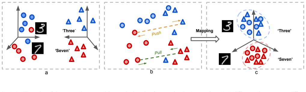
The central machinery is the consensus feature space built by two deep encoders (a CNN for images and a fully connected network for text), trained with the pull-push objective in Eq. (8). The pull term minimizes $1 - \cos(f(M_A^i), g(M_B^j))$ for positive pairs (same class label), while the push term applies the hinge penalty $\max(0, \cos(\cdot) - \gamma)$ for negative sampled pairs (different labels). At test time, Algorithm 2 computes the cosine similarity $F(M_A^i, M_B^i)$ between the two views of the same instance and flags it as an anomaly if this value is below $\epsilon$. The geometry created by the pull-push loss is what makes the single-threshold test work.
What would settle it
Take a dataset where a human annotator labels genuine cross-modal inconsistencies that are not class-label mismatches—for example, two images of the same object that disagree in style, or transactions where profile and behavior conflict—and check whether CMAD's single-threshold cosine-similarity test separates them from normal instances; if precision and recall stay near chance at every threshold, the framework's core mechanism would be refuted.
Extended reading notes
Core claim
The central claim is that cross-modal anomalies can be detected by a threshold test in a learned consensus space, provided the space is trained with a pull-push objective that uses class labels to define consistency. The authors define an instance as anomalous when $F(M_A^i, M_B^i) < \epsilon$, where $F$ is cosine similarity between deep embeddings of its two modalities. To learn the embedding, they minimize for positive pairs (same class labels) the loss $1 - F$ and for negative sampled pairs (different labels) a hinge loss $\max(0, F - \gamma)$. This geometry—consistent views close, inconsistent views far—is what makes the single-threshold test work. The experiments on MNIST and RGB-D support the claim that deep nonlinear encoders capture these cross-modal correlations better than linear CCA-style projections or simpler embedding networks.
Load-bearing premise
The training signal and the test definition both assume that cross-modal anomaly equals a class-label mismatch between modalities, and without class labels for all modalities the method cannot be trained.
Editorial extensions
If this is right
- Anomalies that are invisible when each modality is examined alone become detectable by comparing the same instance across modalities in the learned consensus space.
- Deep nonlinear encoders are necessary: linear CCA, kernel CCA, PLS, and HOAD all underperform CMAD on both datasets, indicating that shallow correlation models miss the complex cross-modal structure.
- The pull-push objective extends to more than two modalities by adding pairwise loss terms, a direct extension the paper states.
- The threshold-based test in Algorithm 2 is computationally cheap, making real-time screening of cross-modal inconsistencies feasible in applications like fraud detection.
- The method requires class labels for every modality during training; without labels, the positive and negative pair sets cannot be constructed, so the approach is supervised.
Reading between the lines
- The reported evaluations inject anomalies as exactly class-label mismatches via negative sampling, so the accuracy figures measure detection of that particular synthetic inconsistency; real-world cross-modal anomalies that are not simple label disagreements remain untested, and the method's transfer to them is an open question.
- When labels are scarce, one could replace the class-label pairing with self-supervised signals such as cross-modal nearest-neighbor consistency or augmented-view agreement, though the paper does not explore this direction.
- The pull-push objective is a form of metric learning; adopting triplet mining or adaptive margin scheduling could improve sample efficiency and stability on larger or noisier datasets.
- Because the anomaly decision is a single threshold on cosine similarity, calibrating epsilon per modality pair (for instance, image-to-image versus image-to-text) may be needed in practice; the paper tunes epsilon per dataset but leaves automatic calibration unaddressed.
Signed reviews
Editorial analysis
A structured set of objections, weighed in public.
Referee Report
Summary. The paper proposes CMAD, a deep structured framework for cross-modal anomaly detection. The method projects each modality through a deep network into a shared latent space and trains with a contrastive loss (Eq. (8)) that pulls together cross-modal pairs whose class labels agree and pushes apart pairs whose labels disagree. At test time, an instance is declared anomalous if the cosine similarity between its two modality embeddings falls below a threshold (Algorithm 2). Experiments on MNIST (with synthetic text tags) and RGB-D inject anomalies via negative sampling, i.e., by pairing modalities with different class labels, and report high accuracy, precision, and recall, including 0.9921 accuracy on MNIST and 0.9512 on RGB-D.
Significance. If the empirical claims held, the paper would make a useful contribution by framing cross-modal anomaly detection as a representation-learning problem and applying deep nonlinear mappings, a clear improvement over linear CCA-style baselines. The objective in Eq. (8) is well specified and the algorithm (Algorithms 1 and 2) is implementable. However, the evaluation protocol is the main weakness: anomalies are constructed by the same label-mismatch rule that defines the supervised training signal, making the reported accuracy a measure of how well the model reproduces the label-pairing rule rather than its ability to detect general cross-modal inconsistencies. The lack of statistical validation and test-set hyperparameter tuning further undermines the central empirical claim. The method may be effective for detecting class-label mismatches, but the paper's broader claims about real-world anomalies such as identity fraud are not supported by the current evidence.
major comments (3)
- [Section IV-A and Eq. (8)] The test anomalies are generated by exactly the same rule used to define the negative training pairs. Section IV-A states that inconsistent pairs are created by randomly sampling pairs {p,q} with y_p^A != y_q^B, which is the definition of the negative set N in Eq. (8). Since the loss in Eq. (8) explicitly trains F to be low for such pairs, and the anomaly score in Algorithm 2 is F itself, the reported accuracy measures the model's ability to reproduce the label-mismatch rule used to construct both its supervision and its ground truth. This is circular with respect to the claim of general cross-modal anomaly detection: real-world anomalies described in the introduction (e.g., identity fraud where the profile does not match the signature) are not defined solely by class-label disagreement, and the paper provides no evidence that the approach transfers to such settings. An evaluation with anomalies defined independently of the training labels is needed to support the central claim.
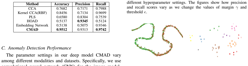
- [Tables II and III; Section IV-D] All results are reported as single numbers without error bars, multiple runs, or significance tests. The injected anomaly counts are small (1,019 for MNIST, 545 for RGB-D), and deep network training is stochastic, so the reported margins over the Embedding Network baseline cannot be evaluated without variance estimates. More seriously, Section IV-D tunes the threshold epsilon and margin gamma directly on the test set, reporting the best accuracy achieved at epsilon=0.3 and gamma=0.3. Since epsilon is the decision threshold in Algorithm 2, selecting it on the test data likely inflates the reported detection accuracy. The authors should use a validation split for hyperparameter selection and report mean and standard deviation over multiple random seeds and injected anomaly sets.
- [Section III-B, Eq. (8) vs. Algorithm 2] The training pairs in S and N are defined between two different instances (i,j) or (p,q), whereas the anomaly score in Algorithm 2 is computed on the two modalities of the same instance, F(M_A^i, M_B^i). The manuscript does not explain why the same-instance similarity is expected to be well calibrated by a training objective that operates on cross-instance pairs. If same-instance modality pairs are not representative of the training pair distribution, the threshold epsilon chosen in Section IV-D may not transfer to the actual detection task. The paper should clarify whether same-instance pairs are included in S or N during training, or otherwise justify the calibration step.
minor comments (4)
- [Section III-B, paragraph 4] The sentence describing the deep framework states that 'instance pairs with consistent patterns across different modalities are pushed away while the pairs with inconsistent cross-modal patterns are pulled together.' This is the opposite of the objective in Eq. (8) and of the rest of the paper; it should read 'pulled together' for consistent patterns and 'pushed away' for inconsistent ones.
- [Section IV-A, Eq. (1) and Algorithm 2] The definition in Eq. (1) uses the condition F < epsilon for an anomaly, while Algorithm 2 writes 'if F(M_A^i, M_B^i) - epsilon < 0'. These are equivalent but the notational inconsistency should be harmonized.
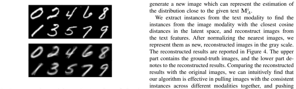
- [Section IV-E, Eq. (12)] Eq. (12) reuses the threshold epsilon as a binarization threshold for weighting neighbor images in the reconstruction case study, but it is unclear whether this is the same epsilon used in Algorithm 2 or a separately tuned value; this should be clarified.
- [Table I] The caption contains a typo: 'Hyaperparameters' should be 'Hyperparameters'.
Circularity Check
High accuracy reflects the same label-mismatch rule used for training and test; detection reduces to thresholding the trained objective.
-
self definitional
[Section III-A Definition (Eq. 1), Section III-B (Eq. 8), Algorithm 2]
"F (Mi A, Mi B)<ϵ, (1) ... we regard that the ith instance is normal across the two modalities; otherwise, the ith instance is a cross-modal anomaly. ... if F (Mi A, Mi B)−ϵ< 0 then the ith instance is a cross-modal anomaly;"
The anomaly score F is the same cosine similarity that the training loss in Eq. (8) directly minimizes for positive pairs and maximizes for negative pairs. Algorithm 2 then thresholds this same F at test time, so the detection outcome is a direct read-out of the training objective. Since the training loss is defined over exactly the same function used to define anomalies in Eq. (1), the 'prediction' that inconsistent patterns have low F is true by construction rather than by independent inference.
-
fitted input called prediction
[Section IV-A (Datasets) and Section III-B (negative set N in Eq. (8))]
"To generate the cross-modal anomalies, we adopt a widely used injection method - negative sampling, to create a number of instance pairs such that their patterns are inconsistent across different modalities. ... we randomly sample a number of k instance pairs {p,q} such that their cross-modal patterns are different such that y_p^A ≠ y_q^B. ... N ={(p,q)} be the set of the negative samples where their cross-modal patterns are inconsistent (i.e., y_p^A ≠ y_q^B)."
The test anomalies are generated by the same label-mismatch rule y_p^A ≠ y_q^B that defines the negative training pairs in Eq. (8). The ground-truth anomalous instances are therefore produced from the same supervision signal the model was explicitly trained to separate. Reported accuracies, including 0.9921 on MNIST and 0.9512 on RGB-D, measure how well the model reproduces this label-pairing rule on held-out pairs, not its ability to detect a broader class of cross-modal inconsistencies such as the bank-fraud or identity-mismatch examples described in the introduction.
full rationale
The paper's central empirical claim is partially circular because the anomaly definition, training objective, detection threshold, and test-injection rule all use the same ingredients. Eq. (1) defines anomalies as instances with low cross-modal similarity F; Eq. (8) trains the network to make F high for same-label pairs and low for different-label pairs; Algorithm 2 thresholds F; and Section IV-A constructs ground-truth anomalies from random pairs with different labels, exactly the negative-sampling rule used for training. Thus the test set does not provide an independent definition of 'cross-modal anomaly' beyond the training signal, and the strong accuracy numbers largely reflect alignment between supervision and ground-truth generation rather than a verified general anomaly-detection capability. The relative comparison against supervised baselines using the same protocol may still be informative as a methodology benchmark, and the self-citations in the references are peripheral rather than load-bearing. However, because the central 'prediction' reduces by construction to the training objective and the test definition, a score of 6 is appropriate.
Assumptions & free parameters
free parameters (5)
- Margin gamma =
0.3 (best on MNIST)
- Threshold epsilon =
0.3 (best on MNIST)
- Lambda (loss weight) =
1
- Network layer dimensions =
784-1440-1280-320-150-50 for MNIST images
- Number of injected anomalies =
1019 (MNIST), 545 (RGB-D)
assumptions (4)
- domain assumption Class labels y_i^k are available for every instance in every modality during training.
- domain assumption Anomalies in the test set are instances whose two modalities have different class labels.
- domain assumption A deep neural network with enough capacity can learn a consensus space where cosine similarity reflects label agreement.
- domain assumption Cosine similarity is an appropriate measure of cross-modal consistency.
Cite this review
Pith. "Pith review of Deep Structured Cross-Modal Anomaly Detection." pith.science (2026). https://pith.science/paper/4OIBBNBL
@misc{pith2026190803848,
  author       = {Pith},
  title        = {Pith review of: Deep Structured Cross-Modal Anomaly Detection},
  year         = {2026},
  howpublished = {\url{https://pith.science/paper/4OIBBNBL}},
  note         = {Machine review of arXiv:1908.03848}
}
read the original abstract
Anomaly detection is a fundamental problem in data mining field with many real-world applications. A vast majority of existing anomaly detection methods predominately focused on data collected from a single source. In real-world applications, instances often have multiple types of features, such as images (ID photos, finger prints) and texts (bank transaction histories, user online social media posts), resulting in the so-called multi-modal data. In this paper, we focus on identifying anomalies whose patterns are disparate across different modalities, i.e., cross-modal anomalies. Some of the data instances within a multi-modal context are often not anomalous when they are viewed separately in each individual modality, but contains inconsistent patterns when multiple sources are jointly considered. The existence of multi-modal data in many real-world scenarios brings both opportunities and challenges to the canonical task of anomaly detection. On the one hand, in multi-modal data, information of different modalities may complement each other in improving the detection performance. On the other hand, complicated distributions across different modalities call for a principled framework to characterize their inherent and complex correlations, which is often difficult to capture with conventional linear models. To this end, we propose a novel deep structured anomaly detection framework to identify the cross-modal anomalies embedded in the data. Experiments on real-world datasets demonstrate the effectiveness of the proposed framework comparing with the state-of-the-art.
Figures

Figures from the paper (1 more)
Reference graph
Works this paper leans on
-
[1]
V . Chandola, A. Banerjee, and V . Kumar, “Anomaly detection: A survey,” ACM computing surveys (CSUR) , vol. 41, no. 3, p. 15, 2009
work page 2009
-
[2]
Muvir: Multi-view rare category detection
D. Zhou, J. He, K. S. Candan, and H. Davulcu, “Muvir: Multi-view rare category detection.” in IJCAI, 2015, pp. 4098–4104
work page 2015
-
[3]
A spectral framework for detecting inconsistency across multi-source object re- lationships,
J. Gao, W. Fan, D. Turaga, S. Parthasarathy, and J. Han, “A spectral framework for detecting inconsistency across multi-source object re- lationships,” in Data Mining (ICDM), 2011 IEEE 11th International Conference on. IEEE, 2011, pp. 1050–1055
work page 2011
- [4]
-
[5]
Kernel and nonlinear canonical correlation analysis,
P. L. Lai and C. Fyfe, “Kernel and nonlinear canonical correlation analysis,” International Journal of Neural Systems , vol. 10, no. 05, pp. 365–377, 2000
2000
-
[6]
Multi-view low-rank analysis for outlier detection,
S. Li, M. Shao, and Y . Fu, “Multi-view low-rank analysis for outlier detection,” in Proceedings of the 2015 SIAM International Conference on Data Mining . SIAM, 2015, pp. 748–756
work page 2015
-
[7]
Collaborative multi-view denoising,
L. Zhang, S. Wang, X. Zhang, Y . Wang, B. Li, D. Shen, and S. Ji, “Collaborative multi-view denoising,” in Proceedings of the 22nd ACM SIGKDD International Conference on Knowledge Discovery and Data Mining. ACM, 2016, pp. 2045–2054
work page 2016
-
[8]
Neural fraud de- tection in credit card operations,
J. R. Dorronsoro, F. Ginel, C. Sgnchez, and C. Cruz, “Neural fraud de- tection in credit card operations,” IEEE transactions on neural networks, vol. 8, no. 4, pp. 827–834, 1997
work page 1997
Show all 32 references
-
[9]
A survey of data mining and machine learning methods for cyber security intrusion detection,
A. L. Buczak and E. Guven, “A survey of data mining and machine learning methods for cyber security intrusion detection,” IEEE Commu- nications Surveys & Tutorials , vol. 18, no. 2, pp. 1153–1176, 2016
2016
-
[10]
A survey on wearable sensor- based systems for health monitoring and prognosis,
A. Pantelopoulos and N. G. Bourbakis, “A survey on wearable sensor- based systems for health monitoring and prognosis,” IEEE Transactions on Systems, Man, and Cybernetics, Part C (Applications and Reviews) , vol. 40, no. 1, pp. 1–12, 2010
2010
-
[11]
Anomaly detection and classification for hyperspectral imagery,
C.-I. Chang and S.-S. Chiang, “Anomaly detection and classification for hyperspectral imagery,” IEEE transactions on geoscience and remote sensing, vol. 40, no. 6, pp. 1314–1325, 2002
2002
-
[12]
Combining negative selection and classification techniques for anomaly detection,
F. Gonzalez, D. Dasgupta, and R. Kozma, “Combining negative selection and classification techniques for anomaly detection,” in Evolutionary Computation, 2002. CEC’02. Proceedings of the 2002 Congress on , vol. 1. IEEE, 2002, pp. 705–710
2002
-
[13]
Intrusion detection with unlabeled data using clustering,
L. Portnoy, E. Eskin, and S. Stolfo, “Intrusion detection with unlabeled data using clustering,” in In Proceedings of ACM CSS Workshop on Data Mining Applied to Security (DMSA-2001 . Citeseer, 2001
2001
-
[14]
Specae: Spectral autoen- coder for anomaly detection in attributed networks,
Y . Li, X. Huang, J. Li, M. Du, and N. Zou, “Specae: Spectral autoen- coder for anomaly detection in attributed networks,” 2019
2019
-
[15]
Clustering- based anomaly detection in multi-view data,
A. Marcos Alvarez, M. Yamada, A. Kimura, and T. Iwata, “Clustering- based anomaly detection in multi-view data,” in Proceedings of the 22nd ACM international conference on Conference on information & knowledge management. ACM, 2013, pp. 1545–1548
2013
-
[16]
Exploiting similarities among languages for machine translation,
T. Mikolov, Q. V . Le, and I. Sutskever, “Exploiting similarities among languages for machine translation,” arXiv preprint arXiv:1309.4168 , 2013
2013 arXiv
-
[17]
Multimodal deep learning,
J. Ngiam, A. Khosla, M. Kim, J. Nam, H. Lee, and A. Y . Ng, “Multimodal deep learning,” in Proceedings of the 28th international conference on machine learning (ICML-11) , 2011, pp. 689–696
2011
-
[18]
Efficient learning of deep boltz- mann machines,
R. Salakhutdinov and H. Larochelle, “Efficient learning of deep boltz- mann machines,” in Proceedings of the thirteenth international confer- ence on artificial intelligence and statistics , 2010, pp. 693–700
2010
-
[19]
Speech recognition with deep recurrent neural networks,
A. Graves, A.-r. Mohamed, and G. Hinton, “Speech recognition with deep recurrent neural networks,” in Acoustics, speech and signal pro- cessing (icassp), 2013 ieee international conference on . IEEE, 2013, pp. 6645–6649
2013
-
[20]
Graph recurrent networks with attributed random walks,
X. Huang, Q. Song, Y . Li, and X. Hu, “Graph recurrent networks with attributed random walks,” 2019
2019
-
[21]
Is a single vector enough? exploring node polysemy for network embedding,
N. Liu, Q. Tan, Y . Li, H. Yang, J. Zhou, and X. Hu, “Is a single vector enough? exploring node polysemy for network embedding,”arXiv preprint arXiv:1905.10668, 2019
1905 arXiv
-
[22]
Dropout: a simple way to prevent neural networks from over- fitting,
N. Srivastava, G. Hinton, A. Krizhevsky, I. Sutskever, and R. Salakhut- dinov, “Dropout: a simple way to prevent neural networks from over- fitting,” The Journal of Machine Learning Research , vol. 15, no. 1, pp. 1929–1958, 2014
1929
-
[23]
MNIST handwritten digit database,
Y . LeCun and C. Cortes, “MNIST handwritten digit database,” 2010. [Online]. Available: http://yann.lecun.com/exdb/mnist/
2010
-
[24]
Distributed representations of words and phrases and their composi- tionality,
T. Mikolov, I. Sutskever, K. Chen, G. S. Corrado, and J. Dean, “Distributed representations of words and phrases and their composi- tionality,” in Advances in neural information processing systems , 2013, pp. 3111–3119
2013
-
[25]
Glove: Global vectors for word representation,
J. Pennington, R. Socher, and C. Manning, “Glove: Global vectors for word representation,” in Proceedings of the 2014 conference on empirical methods in natural language processing (EMNLP) , 2014, pp. 1532–1543
2014
-
[26]
A large-scale hierarchical multi- view rgb-d object dataset,
K. Lai, L. Bo, X. Ren, and D. Fox, “A large-scale hierarchical multi- view rgb-d object dataset,” in Robotics and Automation (ICRA), 2011 IEEE International Conference on . IEEE, 2011, pp. 1817–1824
2011
-
[27]
A kernel method for canonical correlation analysis,
S. Akaho, “A kernel method for canonical correlation analysis,” arXiv preprint cs/0609071, 2006
2006 arXiv
-
[28]
Partial least square regression (pls regression),
H. Abdi, “Partial least square regression (pls regression),” Encyclopedia for research methods for the social sciences , vol. 6, no. 4, pp. 792–795, 2003
2003
-
[29]
Learning two-branch neural networks for image-text matching tasks,
L. Wang, Y . Li, J. Huang, and S. Lazebnik, “Learning two-branch neural networks for image-text matching tasks,” IEEE Transactions on Pattern Analysis and Machine Intelligence , 2018
2018
-
[30]
Learning deep structure-preserving image-text embeddings,
L. Wang, Y . Li, and S. Lazebnik, “Learning deep structure-preserving image-text embeddings,” in Proceedings of the IEEE conference on computer vision and pattern recognition , 2016, pp. 5005–5013
2016
-
[31]
Deep structured energy based models for anomaly detection,
S. Zhai, Y . Cheng, W. Lu, and Z. Zhang, “Deep structured energy based models for anomaly detection,” arXiv preprint arXiv:1605.07717, 2016
2016 arXiv
-
[32]
Heterogeneous network embedding via deep architectures,
S. Chang, W. Han, J. Tang, G.-J. Qi, C. C. Aggarwal, and T. S. Huang, “Heterogeneous network embedding via deep architectures,” in Proceedings of the 21th ACM SIGKDD International Conference on Knowledge Discovery and Data Mining . ACM, 2015, pp. 119–128
2015
Reviewed August 14, 2026 · model on record in the stance chip above.
Discussion (0). Continue with ORCID to comment.