REVIEW 2 major objections 3 minor 24 references
A general model for vegetation patterns including rhizome growth
T0 review · 2 major / 3 minor · reviewed 2026-08-14 · deepseek-v4-flash
Pith's one-line read The paper claims that one scalar PDE, with a gradient-squared term for rhizome elongation, reproduces the full phase diagram and pattern dynamics of a detailed model of clonal plants.
desk verdict Useful reduction of the ABD seagrass model to a single PDE, with a genuinely new |∇n|^2 term, but the signature term's derivation leans on a closure checked on only one stationary pattern. read the letter →
The pith
A machine-rendered reading of the paper's core claim, the machinery that carries it, and where it could break.
The reading
What carries the argument
The machinery is the single PDE for total vegetation density $n(\mathbf{r},t)$ together with the derivation chain that connects it to the angle-resolved ABD model. The new term $\delta\|\nabla n\|^2$ carries the clonal mechanism: unlike linear diffusion $\epsilon\nabla^2 n$, which spreads density down gradients, this term feeds growth from the existence of a gradient and therefore pushes vegetation into empty space. To obtain it, the authors truncate the angular Fourier series of apex density to the first mode, assume the homogeneous steady-state relation between apex and total density holds locally (the weakest step), let the phase relax so apex flux points opposite the density gradient, close the first-mode amplitude as $-(c_0+c_1 n)\nabla n$, and expand the nonlocal interaction kernel in gradients up to fourth order. Each term of Eq. (1) is then expressed in terms of biologically measurable rates: mortality, branching rate and angle, rhizome velocity, shoot spacing, and kernel moments.
What would settle it
Run the full angle-resolved ABD model in the regime where the reduced equation predicts traveling stripes (low branching angle, large $\delta$) and track the local ratio of apex density to total density over time. If that ratio departs systematically from the constant $\eta$ used in the reduction, the derivation of the $\delta\|\nabla n\|^2$ term does not carry over to the moving-pattern regime, and the parity-breaking prediction of the reduced model loses its stated microscopic basis.
Extended reading notes
Core claim
The central claim is that Eq. (1), $\partial_t n = -\omega n + a n^2 - b n^3 + \epsilon\nabla^2 n + \alpha(\nabla^2 n)n + \delta\|\nabla n\|^2 + \beta(\nabla^4 n)n$, is the generic continuum description of clonal-plant pattern formation, with the $\delta\|\nabla n\|^2$ term being the distinctive mark of rhizome growth. The term emerges from the ABD model because clonal propagation creates a biomass flux directed against the density gradient; expanding that flux gives the gradient-squared contribution alongside ordinary and nonlinear diffusion. The paper verifies that the reduced equation reproduces the qualitative behavior of the full model: subcritical coexistence between vegetated and bare states, a modulation (Turing) instability, the same ordering of negative hexagons, stripes, positive hexagons, and localized structures as mortality varies, and, for sufficiently large $\delta$, a parity-breaking bifurcation to traveling stripes that the detailed model also shows at low branching angles.
Load-bearing premise
The argument rests on assuming that the balance between rhizome tips (growing points) and total shoots, a constant measured in uniform steady meadows, stays the same locally even when vegetation is patchy and changing over time; the paper checks this only on a single static pattern, finding errors below 10% of the tip density.
Editorial extensions
If this is right
- Modelers of clonal vegetation can drop the angular coordinate of rhizome growth and still get the correct pattern selection and colonization dynamics, provided the coefficient $\delta$ is set from rhizome speed and branching angle.
- Larger $\delta$ shifts the Maxwell point to higher mortality, so a clonal species should be able to invade bare ground under conditions where a seed-dispersal-only species with identical local dynamics cannot.
- At low branching angles the effective $\delta$ rises, and the model predicts that stationary striped meadows become traveling bands via a parity-breaking instability.
- The parameter mapping gives a direct biological reading of each term: mortality minus branching sets $\omega$, rhizome speed and branching angle set $\epsilon$ and $\delta$, and the kernel moments set $\alpha$ and $\beta$.
- The same sequence of pattern types observed in the detailed model, from bare soil and isolated patches to stripes and labyrinthine patterns, is recovered as mortality is increased.
Reading between the lines
- Because the derivation relies only on rotational symmetry and low-order expansions, the same equation with $\delta>0$ might describe other expanding populations whose local growth is promoted by density gradients, such as fungal colonies or clonal animals, with parameters reinterpreted.
- The closure $N_a=\eta n_t$ is the untested hinge for nonstationary dynamics; a direct check in the traveling-stripe regime, which the paper does not perform, would either secure the reduction or force a state-dependent $\eta$.
- The paper's quantitative link to real seagrass meadows remains indirect: one could measure the front-velocity shift and the traveling-stripe threshold in a real meadow and compare the inferred $\delta$ with the value predicted from branching angle and rhizome speed.
- The model suggests that monitoring the motion of vegetation band edges, not just their shape, could reveal the strength of clonal propagation in the field.
Signed reviews
Editorial analysis
A structured set of objections, weighed in public.
Referee Report
Summary. The paper proposes a single scalar reaction-diffusion PDE, Eq. (1), for vegetation density in clonal-plant meadows, with the new term δ||∇n||² interpreted as the signature of clonal (rhizome) growth. The model is first motivated heuristically by symmetry and positivity requirements, then derived from the microscopic ABD model under a sequence of approximations: angular Fourier truncation, a local closure relating apex density to total density, a truncation of the moment expansion of the nonlocal interaction kernel, and a linear-in-n_t expansion of the saturating interaction. The authors analyze homogeneous steady states, the modulation instability, stationary and localized patterns, front velocities via a perturbative calculation, and traveling patterns for large δ. They claim the reduced model reproduces all qualitative features of the ABD phase diagram and that the δ term accelerates fronts and can induce parity-breaking traveling patterns.
Significance. If the derivation is sound, Eq. (1) provides a valuable minimal descriptor for pattern formation in clonal vegetation, connecting a biologically interpretable coefficient δ to rhizome branching dynamics and making a falsifiable prediction about clonal-growth effects on front propagation. The paper is strong in presenting an explicit derivation chain: the heuristic symmetry argument is independent of the ABD model, the angular-mode truncation is stated as an approximation, and the linear stability and front-velocity calculations are internally consistent and checked against numerical simulations. The perturbative calculation of the δ-induced front-velocity shift is a useful contribution. However, the central new term rests on a closure assumption that is validated only in a single stationary pattern, while the term's claimed effects are demonstrated in moving-front and traveling-pattern regimes where that validation does not directly apply.
major comments (2)
- [Appendix, after Eq. (A7)] The local closure N_a = η n_t (Eq. A6) is derived from the populated homogeneous steady state and then assumed 'valid for all r and t in any heterogeneous spatial distribution.' The only numerical evidence offered is that the maximum error in a stationary pattern is less than 10% of the apex density. This is not sufficient to support the subsequent use of the resulting flux term, which drives the δ||∇n||² signature, in the front-velocity calculation of §V/Fig. 3 and the traveling-pattern regime of Fig. 4. In those regimes the balance ω_b = ω_d that yields Eq. (A6) does not hold. I request either direct numerical tests of the closure in a moving front and a traveling pattern, or a revised claim that restricts the δ signature to stationary configurations.
- [Appendix, Eqs. (A12)-(A16)] The coefficients c0 and c1 are calibrated at the Maxwell point of a stationary front, and the amplitude of the first angular mode is assumed to be a linear function of n_t only, C = c0 + c1 n_t. The relaxation timescale of the angle θ to its fixed point θ = γ + π in Eq. (A10) is not compared with the timescale of front motion, so the quasi-static elimination of the angular dynamics is not established in the regimes where the δ term matters. Moreover, the reported 10% error bound is on the apex density N_a, not on the flux term -ν∇·a' or on δ; even in the stationary test, an error in N_a does not directly bound the error in the gradient-dependent flux that produces δ||∇n||². The quantitative content of the new term therefore remains unsupported away from the Maxwell point. Please provide an error estimate for the flux term or additional numerical checks of C(nt,∇nt) in moving and time-dependent solutions.
minor comments (3)
- [Section IV, first paragraph] The statement that b = 1 and β = -1 are set 'without loss of generality' implicitly requires β < 0. For the rescalings to be real, the sign of β must be fixed; please state the sign condition or discuss the β > 0 case.
- [Section IV, Fig. 2] The claim that the phase diagram reproduces the ABD model is supported only by a reference to Fig. S3 of Ref. [5]. A direct overlay of the pattern-existence boundaries or a side-by-side comparison would make the claim verifiable within this paper.
- [Section II, after Eq. (1)] The sentence 'A term containing ∇⁴n could in principle be added to Eq. (1), but it does not add any qualitatively new behavior' is confusing because Eq. (1) already contains β(∇⁴n)n. The authors presumably mean a linear ∇⁴n term; please clarify.
Circularity Check
No circularity: the ABD-to-reduced-model reduction is a calibrated consistency check, and the delta-norm-gradient term is not an output forced by its inputs.
full rationale
The paper's central claim is a model reduction, not a circular prediction. Equation (1) is first posed from symmetry and low-order-gradient considerations in Section II, so the target form is not obtained by fitting ABD output. The later derivation from the ABD model in the Appendix fixes the coefficients c0 and c1 from the Maxwell point of the ABD model (Eqs. A14-A16) and then defines delta = nu*c1, so the reduced equation's parameters are calibrated to the source model. The subsequent claims, such as the front-velocity shift (Fig. 3) and the pattern sequence (Figs. 1-2), are computed from Eq. (1) and compared with ABD only qualitatively, making this a consistency check rather than an output forced by the input. The closure N_a = eta*n_t (Eq. A6) is an approximation for heterogeneous states and is checked numerically to less than 10% in one stationary pattern; the paper explicitly labels this as a second approximation, so it is a support gap, not a circular step. The self-citations (Refs. [5,17]) are to previously published, externally confronted models and do not function as unverified uniqueness theorems. The gradient-squared term is introduced through the low-order closure ansatz (A12), but the paper is explicit that this is a leading-term power expansion, and the term's coefficient is not fitted to the phenomenology it later predicts.
Assumptions & free parameters
free parameters (3)
- c0 =
ν/(2(ωd0,M - ωb cos φb))
- c1 =
ν/(2 n*_t,M) * (1/(ωb cos φb - ωd0,M) - 1/(ωb cos φb - ωb))
- Parameter set for figures (a, b, ε, α, δ, β) =
a=1.39, b=1, ε=1.15e-2, α=-1.78, δ=1.03e-2, β=-1
assumptions (6)
- domain assumption Bare soil (n=0) is always a solution and vegetation density is non-negative
- domain assumption The large-scale equation is rotationally invariant and includes only low-order polynomial and gradient terms
- ad hoc to paper Angular Fourier modes m>1 of the apex density are negligible
- ad hoc to paper The homogeneous steady-state relation N_a = η n_t holds locally in heterogeneous configurations
- ad hoc to paper The saturating interaction exponential can be linearized to first order: 1 - e^{-a_e n} ≈ a_e n
- ad hoc to paper The amplitude of the first angular mode is a linear function of density: C = c0 + c1 n_t, independent of gradients and higher derivatives
Cite this review
Pith. "Pith review of A general model for vegetation patterns including rhizome growth." pith.science (2026). https://pith.science/paper/4SGDPNQ4
@misc{pith2026190804603,
  author       = {Pith},
  title        = {Pith review of: A general model for vegetation patterns including rhizome growth},
  year         = {2026},
  howpublished = {\url{https://pith.science/paper/4SGDPNQ4}},
  note         = {Machine review of arXiv:1908.04603}
}
read the original abstract
Vegetation patterns, a natural phenomenon observed worldwide, are typically driven by spatially distributed feedback. However, the spatial colonization mechanisms of clonal plants, driven by the growth of a rhizome, are usually not considered in prototypical models. Here we propose a general equation for the vegetation density that includes all main clonal-growth features as well as the essential ingredients leading to spatial self-organization. This generic model reproduces the phase diagram of a fully detailed model of clonal growth. The relation of each term of the model with the mechanisms of clonal growth is discussed.
Figures


Reference graph
Works this paper leans on
-
[5]
D. Ruiz-Reyn´ es, D. Gomila, T. Sintes, E. Hern´ andez- Garc ´ ıa, N. Marb` a, and C. M. Duarte, Science Advances 3, e1603262 (2017)
work page 2017
-
[1]
This will allow us to give a one to one correspondence of the parameters in Eq
Derivation of the clonal-growth equation We derive here our simplified equation for the spatial distribution of the density n(⃗ r, t) of clonal-growth vege- tation: ∂tn = −ωn + an2 − bn3 + ǫ∇2n + α(∇2n)n + δ‖⃗∇n‖ 2 + β(∇4n)n , (A1) 6 starting from the more detailed and biologically moti- vated ABD model [5]. This will allow us to give a one to one correspo...
-
[2]
0 max(n) T M I FIG. 1. Bifurcation diagram of the homogeneous steady states n∗ (red lines) and stationary patterns of Eq. (1). The maximum value of the density n(⃗ r) is plotted as a function of mortality ω. Solid (dashed) lines indicate stable (unsta- ble) solutions. The 2 d spatial distribution of each solution is shown in the corresponding inset: negat...
-
[3]
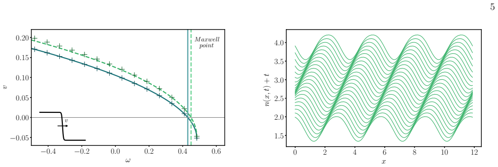
20 v M axwell point v FIG. 3. Velocity of a front between bare-soil and the homo- geneous populated solution (in the absence of the MI) as a function of the mortality ω. Crosses are the results of nu- merical simulations. The curve in blue (solid) corresponds to the analytical solution of Eq. (1) for α = β = δ = 0 (see Appendix). The curve in green (dashe...
-
[4]
The velocity of the patterns grows, increasing δ
The figure shows a periodic pattern traveling to the right, whereas another solution (with shape related by the x → − x parity transformation) with velocity to- ward the left also exists. The velocity of the patterns grows, increasing δ. Such parity-breaking bifurcation from steady to moving patterns is actually observed in the ABD model for low branching ...
work page 2017
-
[6]
Calculation of the velocity of a front using a perturbative method We consider Eq. (A2) in the case of α = β = 0. Thus, the dispersion relation changes with the wave number q as −ǫq2, the maximum growth rate corresponds to q = 0 and the modulational instability is absent. In this case, solutions consisting of an unpopulated and a populated homogeneous sol...
-
[7]
+ ǫ∂2 x + v0∂x one can write ˆLn1 = −δ(∂xn0)2 − v1∂xn0. (A24) Let ⟨f ⏐ ⏐g⟩ = ∫ ∞ −∞ f (x)g(x)dx be the inner product, ˆL† the adjoint of ˆL, and w(x) = exp ( v0 ǫ x ) ∂xn0 the neutral mode of ˆL† ( ˆL†w = 0). We can apply the solvability con- dition ⟨w ⏐ ⏐ˆLn1⟩ = ⟨w ⏐ ⏐f (x)⟩, so that ⟨ ˆL†w ⏐ ⏐n1⟩ = ⟨w ⏐ ⏐f (x)⟩ and 0 = ⟨w ⏐ ⏐f (x)⟩, to write ⟨w ⏐ ⏐− δ(∂...
-
[8]
Meron, Nonlinear Physics of Ecosystems (CRC Press, Boca Raton, 2015)
E. Meron, Nonlinear Physics of Ecosystems (CRC Press, Boca Raton, 2015)
work page 2015
Show all 24 references
-
[9]
Gowda, H
K. Gowda, H. Riecke, and M. Silber, Physical Review E 89, 022701 (2014)
2014
-
[10]
Rietkerk and J
M. Rietkerk and J. van de Koppel, Trends in Ecology & Evolution 23, 169 (2008)
2008
-
[11]
Getzin, H
S. Getzin, H. Yizhad, B. Bell, T. E. Erickson, A. C. Postle, I. Katra, O. Tzuk, Y. R. Zel- nik, K. Wiegand, T. Wiegand, and E. Meron, Proceedings of the National Academy of Sciences 113, 3551 (2016)
2016
-
[12]
The latter work identified three key ingredients
or through the definition of discrete growth rules [13]. The latter work identified three key ingredients. First, the rhizome of a plant, whose tip is called the apex, grows horizontally at constant velocity ν, leaving behind new shoots separated by a characteristic distance ρ. ...
-
[13]
M. C. Cross and P. C. Hohenberg, Rev. Mod. Phys. 65, 851 (1993)
1993
-
[14]
Lefever and O
R. Lefever and O. Lejeune, 9 Bulletin of Mathematical Biology 59, 263 (1997)
1997
-
[15]
Lejeune and M
O. Lejeune and M. Tlidi, Journal of Vegetation Science 10, 201 (1999)
1999
-
[16]
Lejeune, M
O. Lejeune, M. Tlidi, and P. Couteron, Phys. Rev. E 66, 010901(R) (2002)
2002
-
[17]
Fernandez-Oto, O
C. Fernandez-Oto, O. Tzuk, and E. Meron, Phys. Rev. Lett. 122, 048101 (2019)
2019
-
[18]
P. V. Paulau, D. Gomila, C. L´ opez, and E. Hern´ andez- Garc ´ ıa, Phys. Rev. E89, 032724 (2014)
2014
-
[19]
R. D. Routledge, Journal of Applied Probability 27, 1 (1990)
1990
-
[20]
Sintes, N
T. Sintes, N. Marb` a, C. M. Duarte, and G. A. Kendrick, Oikos 108, 165 (2005)
2005
-
[21]
J. D. Murray, Mathematical Biology I: An Introduc- tion, Vol. 17 of Interdisciplinary Applied Mathematics (Springer, New York, 2002)
2002
-
[22]
A. J. Alvarez-Socorro, M. G. Clerc, G. Gonz´ alez-Cort´es, and M. Wilson, Phys. Rev. E 95, 010202(R) (2017)
2017
-
[23]
L¨ ober, M
J. L¨ ober, M. B¨ ar, and H. Engel, Phys. Rev. E 86, 066210 (2012)
2012
-
[24]
Ruiz-Reyn´ es, and D
D. Ruiz-Reyn´ es, and D. Gomila, Phys. Rev. E 100, 052208 (2019)
2019
Reviewed August 14, 2026 · model on record in the stance chip above.
Discussion (0). Continue with ORCID to comment.