REVIEW 2 major objections 4 minor 28 references
Thermodynamical extension of a symplectic numerical scheme with half space and time shift demonstrated on rheological waves in solids
T0 review · 2 major / 4 minor · reviewed 2026-08-14 · deepseek-v4-flash
Pith's one-line read This paper introduces a staggered half-space, half-time finite-difference scheme for the Poynting–Thomson–Zener rheological solid and argues that at $\alpha=1/2$, $\hat C=1$ it is second-order accurate, stable, and free of dissipative and…
desk verdict A solid staggered finite-difference scheme for PTZ waves with rigorous periodic stability analysis, but the optimal C-hat=1 claim rests on an unproven boundary-condition assumption. read the letter →
The pith
A machine-rendered reading of the paper's core claim, the machinery that carries it, and where it could break.
The reading
What carries the argument
The load-bearing mechanism is the staggered spacetime grid: velocities live at half-integer positions in both space and time relative to stress, strain shares stress's nodes, and temperature is half-shifted in time afterwards, so every discrete derivative is evaluated at the midpoint of the quantity it couples to. This arrangement makes the Hooke-case scheme computationally identical to symplectic Euler, the standard first-order geometric integrator, while raising its accuracy to second order by reflection symmetry, and it turns the PTZ constitutive equation into the explicit weighted update (33) with parameter $\alpha$. Stability is controlled by the eigenvalues of the $3\times 3$ iteration (transfer) matrix, which the paper tests through two classical polynomial root-location criteria; those criteria isolate the parameter-free thermodynamic condition $\hat\tau>\tau$ and the fastest-wave Courant condition, and at $\alpha=1/2$, $\hat C=1$ the eigenvalues collapse to $1$ and $e^{\pm ik\Delta x}$, eliminating numerical dissipation and dispersion up to $O(\Delta t/\tau)$.
What would settle it
For the actual finite sample (stress pulse at one end, free end at the other), assemble the full iteration matrix and compute its eigenvalues at $\alpha=1/2$, $\hat C=1$; any eigenvalue with modulus above 1, or a numerical experiment showing unbounded growth of total energy over many bounces, would falsify the claimed boundary-value stability.
Extended reading notes
Core claim
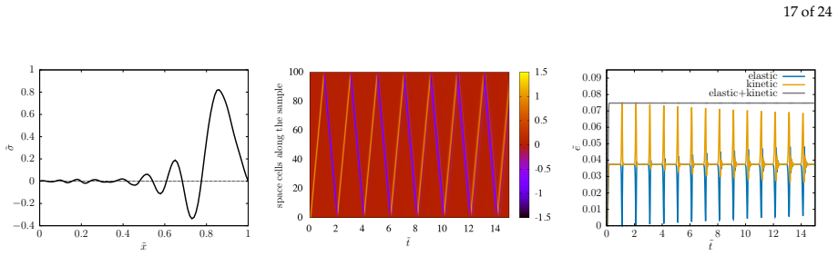
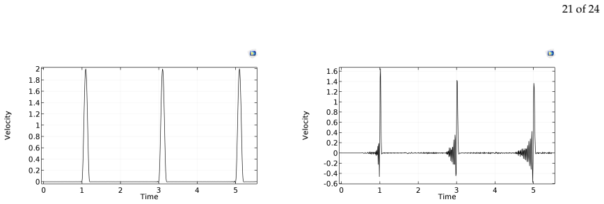
The central discovery is that the PTZ wave system admits a staggered finite-difference realization in which stress, strain, and velocity sit at mutually half-shifted positions dictated by the equations containing them: velocity is half-shifted in both space and time from stress, strain sits with stress, and temperature is then half-shifted in time. The rheological equation, which couples each quantity to its own time derivative, is discretized by an $\alpha$-weighted average that is explicit and second-order accurate at $\alpha=1/2$. A plane-wave stability analysis of the resulting iteration matrix yields three conditions: the thermodynamic requirement $\hat\tau>\tau$, a relation between $\alpha$ and $\Delta t$, and the Courant-type bound $\hat C<1$ (extendable to $\hat C\le 1$ with boundary conditions), where $\hat C=\hat c\,\Delta t/\Delta x$ uses the fast wave speed $\hat c=\sqrt{\hat E/(\tau\varrho)}$. At the special point $\alpha=1/2$, $\hat C=1$, the three eigenvalues that multiply each Fourier mode per time step are exactly $1$ and $e^{\pm ik\Delta x}$, so all wavelengths travel at the same discrete speed and the dissipative and dispersive errors are of order $O(\Delta t/\tau)$. The same scheme applied to the elastic limit conserves total energy over many bounces and produces clean wave pulses where the commercial finite-element software COMSOL, with several tuned time-stepping methods, gives damped, oscillatory, or unstable results and takes 100 to 10,000 times longer.
Load-bearing premise
The load-bearing premise is that stability proved for waves on an infinitely long periodic medium also holds for the finite sample with a stress pulse at one end and a free end, a boundary-value extension the paper treats as a rule of thumb rather than a proof.
Editorial extensions
If this is right
- Setting $\alpha=1/2$ and $\hat C\le 1$ is enough for stability of the PTZ scheme, and with $\hat C=1$ the discrete dispersion branches are linear, so the scheme has no numerical dissipation or dispersion up to $O(\Delta t/\tau)$.
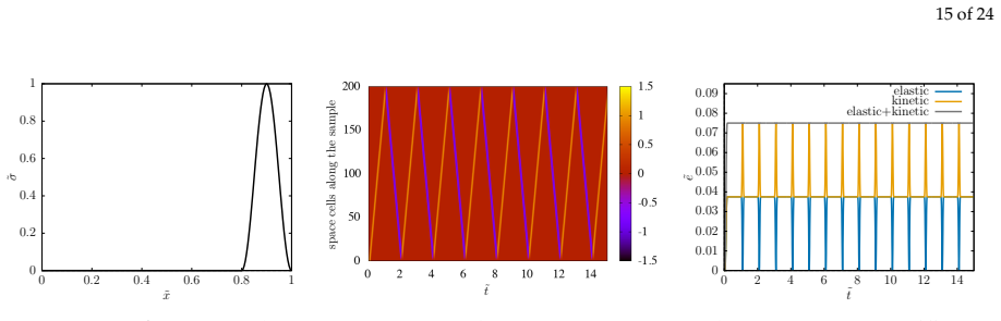
- In the Hooke limit the scheme reduces to symplectic Euler, is stable for $C\le 1$, conserves elastic plus kinetic energy over long times, and needs $C=1$ to avoid both dissipative and dispersive artifacts.
- For the Kelvin–Voigt limit ($\tau=0$) the stability conditions become $\alpha<1/2$ (relaxed to $\alpha\le 1/2$ with boundary conditions) together with a mixed parabolic-hyperbolic Courant bound combining $\Delta t^2$ and $\hat\tau\Delta t$ terms.
- The stability analysis is not purely numerical: it reproduces the thermodynamic stability condition $\hat\tau>\tau$ as a scheme-independent requirement, so numerical stability criteria can teach something about the underlying continuum model.
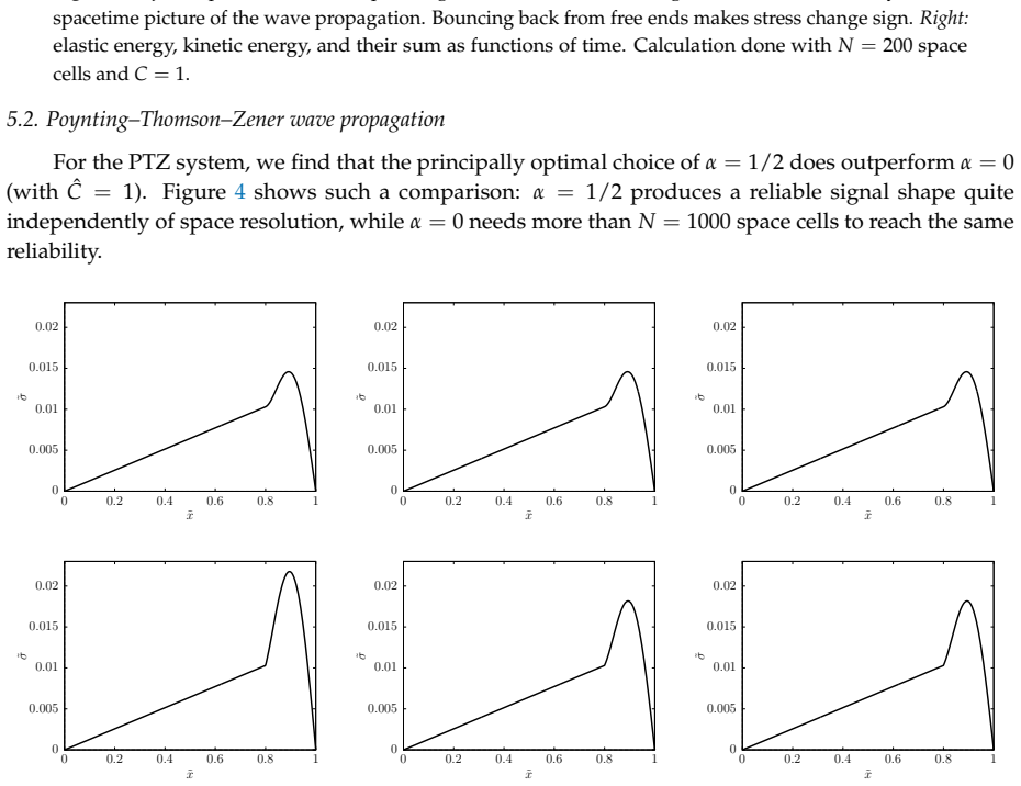
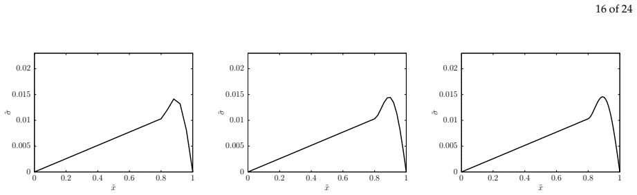
- Practically, the $\alpha=1/2$ scheme gives a reliable PTZ stress-signal shape with as few as 25 to 50 spatial cells, whereas $\alpha=0$ needs more than 1000 cells for comparable quality.
Reading between the lines
- A natural extension, listed by the authors as future work but not demonstrated, is that the same half-shift recipe transfers to other members of the Kluitenberg–Verhás family and to non-Fourier heat conduction, with parabolic limits likely requiring mixed Courant conditions analogous to the Kelvin–Voigt case.
- Because the elastic limit coincides with symplectic Euler, a plausible conjecture the paper does not prove is that the full PTZ scheme inherits a discrete variational or symplectic structure, which would explain the observed total-energy conservation.
- A direct testable extension would be to compare the scheme's temperature histories with an analytic PTZ solution in the force-equilibrial limit; the paper leaves analytic comparison as future work and does not yet provide a convergence study of the thermal field.
- The COMSOL comparison suggests a broader benchmarking lesson: commercial finite-element packages may be unreliable for viscoelastic wave propagation unless the time stepper and tolerances are carefully chosen, so benchmark suites should include dissipative wave problems rather than only static or quasi-static cases.
Signed reviews
Editorial analysis
A structured set of objections, weighed in public.
Referee Report
Summary. The paper presents a staggered finite difference scheme for the one-dimensional Poynting–Thomson–Zener (PTZ) rheological model, building on the symplectic Euler method and extending it to a dissipative continuum system. The authors derive the scheme from a spacetime-staggered arrangement of stress, strain, and velocity, analyze its von Neumann stability for both the Hooke and PTZ cases, and study dissipative and dispersive errors analytically and numerically. They then compare the scheme with COMSOL finite element simulations on a Hookean wave-propagation problem, reporting large run-time and accuracy advantages. The central claims are that the scheme is second-order accurate for α=1/2, that stability is governed by the Courant condition based on the fastest wave speed, and that with α=1/2 and the Courant number at the boundary of the stability region the scheme has linear dispersion branches and suppressed dissipative error.
Significance. If the claims hold, the scheme is a useful, simple, and fast alternative to standard finite element tools for linear rheological wave problems, with the attractive feature that its design follows from the spacetime structure of the governing equations rather than from fitted parameters. The paper contributes a clean, self-contained derivation: no constants are fitted, the Hooke-case stability analysis is rigorous and explicit, and the PTZ stability conditions are derived in closed form via both Jury and Routh–Hurwitz criteria. The explicit demonstration that the thermodynamic condition τ̂>τ emerges from the numerical stability analysis is a nice conceptual point. The COMSOL comparison, though limited to a linear elastic setup, is concrete and reproducible in its setup.
major comments (2)
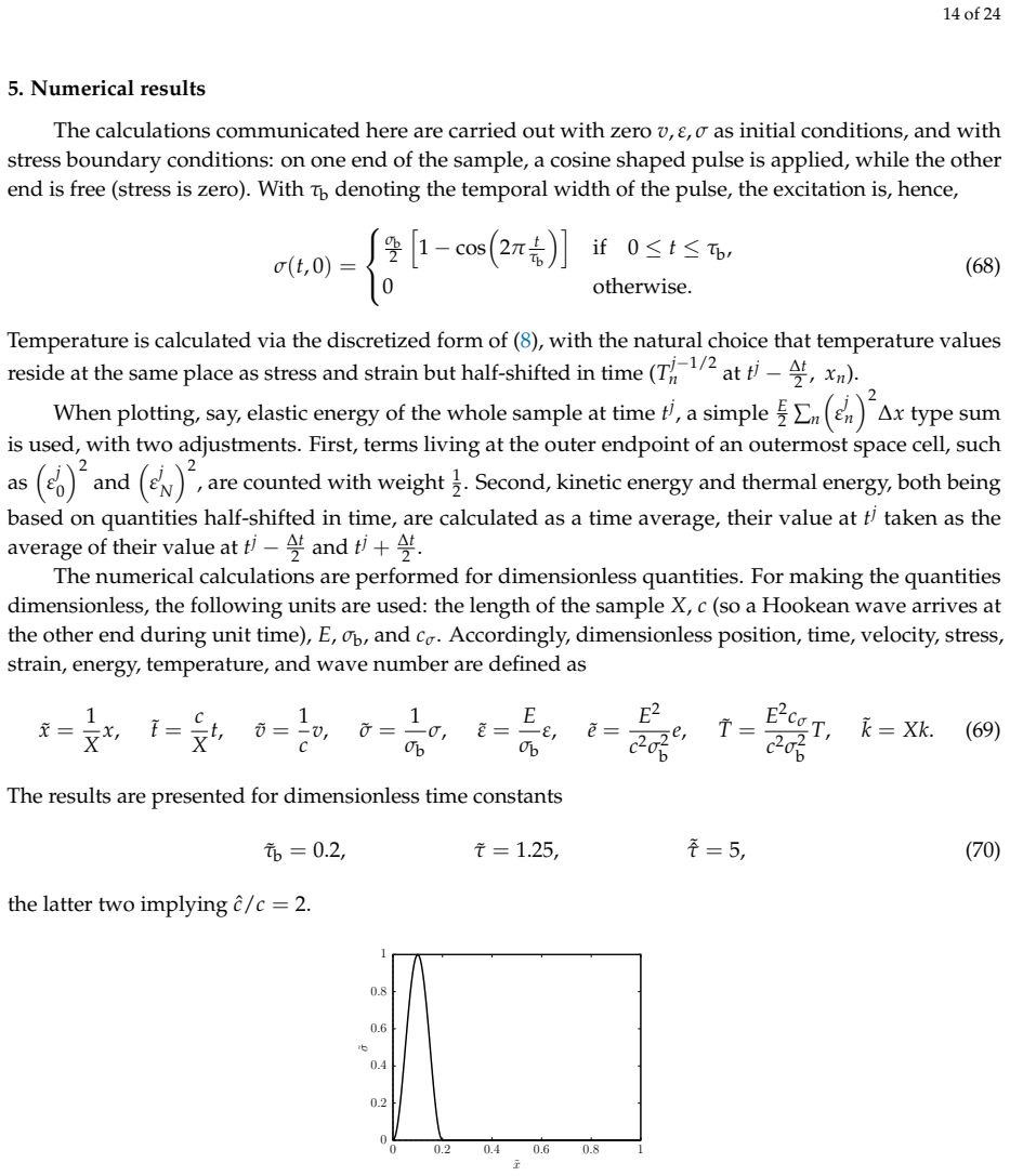
- [Section 4.2.2, Eq. (66)–(67)] The transition from the strict stability condition Ĉ<1 derived in Eq. (60)/(66) to the claimed Ĉ≤1 in Eq. (67) is not proven. The paper explicitly labels this as a rule-of-thumb extension: the von Neumann analysis treats plane waves on an infinite periodic domain, while the actual simulations in Section 5.2 use a finite sample with a stress pulse at one end and a free boundary at the other. The exceptional mode with S=1 (kΔx=π) is precisely where the Jury inequality (60) fails, and the paper does not show that this mode is inadmissible for the pulse/free-boundary problem. Since the headline numerical results are run at Ĉ=1, the advertised stability of the scheme for the reported boundary-value problem rests on an unproven assumption. Please either prove that the exceptional mode is excluded by the boundary conditions, perform a boundary-mode analysis, or revise the stability claim to Ĉ<1 and rerun the key simulations accordingly.
- [Section 3, Eq. (32)–(33)] The claim that α=1/2 renders the PTZ update (33) second-order accurate is asserted without proof. The sentence "Second order accuracy of (33) for α=1/2 is then straightforward to verify" is not sufficient, especially because the update combines a finite difference ratio with an interpolation in σ and ε. The paper's stated advantage over the first-order symplectic Euler method depends on this accuracy claim, so a local truncation error derivation for the rheological update should be included or explicitly referenced. Without it, the accuracy comparison in Section 5.2 and the error discussion in Section 6.2 lack a rigorous basis.
minor comments (4)
- [Section 4.1, after Eq. (46)] There is a typo in the sentence "this affects only one mode, S=1, k=π/k"; this should read "kΔx=π".
- [Section 6.1, Figure 8] The caption of Figure 8 does not indicate whether the upper and lower rows correspond to C=1 and C=1/2, respectively, as stated in the text; the caption should be self-contained.
- [Section 7] The comparison with COMSOL would be more convincing if the exact COMSOL settings (mesh element order, solver tolerances, time-stepping parameters) were listed in a table, since the runtime differences depend strongly on these choices.
- [References] Reference [21] is cited as "in preparation" and "under review"; if the manuscript is being finalized, this reference should either be updated to a published version or removed as a support for the claim about dynamic versus static moduli.
Circularity Check
No circularity found: the scheme, stability analysis, and error analysis are self-contained; the C-hat=1 boundary-condition extension is explicitly a rule-of-thumb, not a circular derivation.
full rationale
The derivation chain is self-contained. The finite-difference scheme is constructed directly from the PTZ equations (1)-(3) by placing v half-shifted in space and time relative to sigma, and epsilon half-shifted relative to v, with the rheological equation discretized by the alpha-weighted formula (32); this is an explicit construction, not an output of the stability analysis. The stability conditions are obtained by computing the transfer matrix (51), its characteristic polynomial (52), and applying Jury/Routh-Hurwitz criteria, yielding (58)-(60). No parameter is fitted to a subset of data and then renamed as a prediction: the only settings (alpha=1/2, C-hat=1) are chosen by the analysis itself. The self-citations to refs [1], [17], and [18] provide the staggered-placement idea and the thermodynamic PTZ model as inputs; they are not used to define away any target claim. The equality extension (67) of the strict condition (66) is explicitly labelled by the authors as a rule-of-thumb (Section 4, paragraph after Eq. (43)), i.e. an unproven assumption about boundary conditions; this is a correctness or assumption limitation, not a circular reduction. The COMSOL comparison is an external benchmark, and the energy conservation check is a non-built-in test. Hence score 0.
Assumptions & free parameters
free parameters (1)
- alpha =
1/2 (optimal for second-order accuracy)
assumptions (3)
- domain assumption The PTZ model (Eqs. 1-3) is a valid continuum thermodynamic model for the solid.
- domain assumption The von Neumann stability criterion (|xi|<=1 for all k) is sufficient for stability of the initial-boundary value problem.
- standard math The Taylor expansion and standard finite difference error analysis are valid.
Cite this review
Pith. "Pith review of Thermodynamical extension of a symplectic numerical scheme with half space and time shift demonstrated on rheological waves in solids." pith.science (2026). https://pith.science/paper/4SM3PCRI
@misc{pith2026190807975,
  author       = {Pith},
  title        = {Pith review of: Thermodynamical extension of a symplectic numerical scheme with half space and time shift demonstrated on rheological waves in solids},
  year         = {2026},
  howpublished = {\url{https://pith.science/paper/4SM3PCRI}},
  note         = {Machine review of arXiv:1908.07975}
}
read the original abstract
On the example of the Poynting-Thomson-Zener rheological model for solids, which exhibits both dissipation and wave propagation - with nonlinear dispersion relation -, we introduce and investigate a finite difference numerical scheme. Our goal is to demonstrate its properties and to ease the computations in later applications for continuum thermodynamical problems. The key element is the positioning of the discretized quantities with shifts by half space and time steps with respect to each other. The arrangement is chosen according to the spacetime properties of the quantities and of the equations governing them. Numerical stability, dissipative error and dispersive error are analysed in detail. With the best settings found, the scheme is capable of making precise and fast predictions. Finally, the proposed scheme is compared to a commercial finite element software, COMSOL, which demonstrates essential differences even on the simplest - elastic - level of modelling.
Figures

Figures from the paper (14 more)





Reference graph
Works this paper leans on
-
[1]
Rieth, Á.; Kovács R.; Fülöp, T. Implicit numerical schemes for generalized heat conduction equations.International Journal of Heat and Mass T ransfer 2018, 126, 1177–1182
work page 2018
-
[2]
Zinner, C.P .; Öttinger, H.C. Numerical stability with help from entropy: Solving a set of 13 moment equations for shock tube problem. Journal of Non-Equilibrium Thermodynamics 2019, 44, 43–69
work page 2019
-
[3]
Structure-preserving integrators for dissipative systems based on reversible-irreversible splitting
Shang, X.; Öttinger, H.C. Structure-preserving integrators for dissipative systems based on reversible-irreversible splitting. Preprint 2018, https://arxiv.org/pdf/1804.05114.pdf
work page Pith review arXiv 2018
-
[4]
Portillo, D.; García Orden, J.C.; Romero, I. Energy-Entropy-Momentum integration schemes for general discrete non-smooth dissipative problems in thermomechanics. International Journal for Numerical Methods in Engineering 2017, 112, 776–802
work page 2017
-
[5]
Contact variational integrators
Vermeeren, M.; Bravetti, A.; Seri, M. Contact variational integrators. Journal of Physics A: Mathematical and Theoretical 2019, 52, 445206
work page 2019
-
[6]
Variational discretization of the nonequilibrium thermodynamics of simple systems
Gay-Balmaz, F.; Yoshimura, H. Variational discretization of the nonequilibrium thermodynamics of simple systems. Nonlinearity 2018, 31, 1673
work page 2018
-
[7]
Variational discretization of thermodynamical simple systems on Lie groups
Couéraud, B.; Gay-Balmaz, F. Variational discretization of thermodynamical simple systems on Lie groups. Discrete & Continuous Dynamical Systems - S 2020, 13, DOI: 10.3934/dcdss.2020064
-
[8]
Romero, I. Algorithms for coupled problems that preserve symmetries and the laws of thermodynamics: Part I: Monolithic integrators and their application to finite strain thermoelasticity. Computer Methods in Applied Mechanics and Engineering 2010, 199, 1841–1858
work page 2010
Show all 28 references
-
[9]
Algorithms for coupled problems that preserve symmetries and the laws of thermodynamics: Part II: fractional step methods
Romero, I. Algorithms for coupled problems that preserve symmetries and the laws of thermodynamics: Part II: fractional step methods. Computer Methods in Applied Mechanics and Engineering 2010, 199, 2235–2248
2010
-
[10]
Internal Variables in Thermoelasticity Springer: Cham, Switzerland, 2017
Berezovski, A.; Ván, P . Internal Variables in Thermoelasticity Springer: Cham, Switzerland, 2017
2017
-
[11]
Janeˇ cka, A.; Málek, J.; Pr ˚ uša, V .; Tierra, G. Numerical scheme for simulation of transient flows of non-Newtonian fluids characterised by a non-monotone relation between the symmetric part of the velocity gradient and the Cauchy stress tensor. Acta Mechanica 2019, 230, 729–747
2019
-
[12]
Elastic, thermal expansion, plastic and rheological processes – theory and experiment
Asszonyi, Cs.; Csatár A.; Fülöp, T. Elastic, thermal expansion, plastic and rheological processes – theory and experiment. Period. Polytech. Civil Eng. 2016, 60, 591–601
2016
-
[13]
Emergence of non-Fourier hierarchies
Fülöp, T.; Kovács, R.; Lovas, Á.; Rieth, Á.; Fodor, T.; Szücs, M.; Ván, P .; Gróf, Gy. Emergence of non-Fourier hierarchies. Entropy 2018, 20, Paper 832
2018
-
[14]
A case study of 3D stress orientation determination in Shikoku Island and Kii Peninsula, Japan
Lin, W.; Kuwahara, Y.; Satoh, T.; Shigematsu, N.; Kitagawa, Y.; Kiguchi, T.; et al. A case study of 3D stress orientation determination in Shikoku Island and Kii Peninsula, Japan. In Proceedings of Eurock’09, Rock Engineering in Difficult Ground Conditions (Soft Rock and Karst)...
2009
-
[15]
Three-dimensional in situ stress determination by anelastic strain recovery of a rock core
Matsuki K.; Takeuchi, K. Three-dimensional in situ stress determination by anelastic strain recovery of a rock core. Int. J. Rock Mech. Min Sci. & Geomech. Abstr. 1993, 30, 1019–1022
1993
-
[16]
Anelastic strain recovery compliance of rocks and its application to in situ stress measurement
Matsuki, K. Anelastic strain recovery compliance of rocks and its application to in situ stress measurement. Int. J. Rock Mech. Min Sci. 2008, 45, 952–965
2008
-
[17]
Analytical solution method for rheological problems of solids
Fülöp, T.; Szücs, M. Analytical solution method for rheological problems of solids. Preprint 2018, https://arxiv. org/pdf/1810.06350.pdf
2018 arXiv
-
[18]
Distinguished rheological models for solids in the framework of a thermodynamical internal variable theory
Asszonyi, Cs.; Fülöp, T.; Ván, P . Distinguished rheological models for solids in the framework of a thermodynamical internal variable theory. Continuum Mech. Thermodyn. 2015, 27, 971–986
2015
-
[19]
Kinematic quantities of finite elastic and plastic deformation
Fülöp, T.; Ván, P . Kinematic quantities of finite elastic and plastic deformation. Mathematical Methods in the Applied Sciences 2012, 35, 1825–1841
2012
-
[20]
Objective thermomechanics
Fülöp, T. Objective thermomechanics. Preprint 2015, https://arxiv.org/pdf/1510.08038.pdf
2015 arXiv
-
[21]
Investigation of relationship between dynamic and static deformation moduli of rocks
Davarpanah, S.M.; Ván P .; Vásárhelyi, B. Investigation of relationship between dynamic and static deformation moduli of rocks. Geomechanics and Geophysics for Geo-Energy and Geo-Resources (under review); talk at GEOMATES 2019 International Congress on Geomathematics in Earth-...
2019
-
[22]
Hairer, E.; Lubich C.; Wanner, G.Geometric Numerical Integration, 2nd ed.; Springer-Verlag: Berlin–Heidelberg, Germany, 2006
2006
-
[23]
Numerical integration of the barotropic vorticity equation
Charney, J.G.; Fjörtoff, R.; von Neumann, J. Numerical integration of the barotropic vorticity equation. T ellus 1950, 2, 237–254
1950
-
[24]
An Introduction to Difference Equations, 3rd ed.; Springer, New York, USA, 2005
Elaydi, S. An Introduction to Difference Equations, 3rd ed.; Springer, New York, USA, 2005
2005
-
[25]
Matolcsi, T. Ordinary Thermodynamics – Nonequilibrium Homogeneous Processes ; Society for the Unity of Science and Technology: Budapest, Hungary, 2017; available at http://energia.bme.hu/~fulop/Matolcsi_Ordinary_ Thermodynamics_2017-04-26.pdf
2017
-
[26]
Von Neumann stability analysis of globally divergence-free RKDG schemes for the induction equation using multidimensional Riemann solvers
Balsara, D.S.; Käppeli, R. Von Neumann stability analysis of globally divergence-free RKDG schemes for the induction equation using multidimensional Riemann solvers. Journal of Computational Physics 2017, 336, 104–127
2017
-
[27]
Inners and Stability of Dynamical Systems , John Wiley & Sons: New York, USA, 1974
Jury, E.I. Inners and Stability of Dynamical Systems , John Wiley & Sons: New York, USA, 1974
1974
-
[28]
Józsa, V .; Kovács, R.Solving Problems in Thermal Engineering – A T oolbox for Engineers , Springer, Germany, 2019 (to appear), DOI: 10.1007/978-3-030-33475-8
2019 doi
Reviewed August 14, 2026 · model on record in the stance chip above.
Discussion (0). Continue with ORCID to comment.