REVIEW 2 major objections 3 minor 13 references
Non-Abelian Gauge-Invariant Cellular Automata
T0 review · 2 major / 3 minor · reviewed 2026-08-14 · deepseek-v4-flash
Pith's one-line read The paper constructs a non-abelian gauge-invariant cellular automaton and characterizes when two such theories are equivalent.
desk verdict Genuine non-abelian gauge-invariant CA construction, but Proposition 4 is false as stated and needs a fix. read the letter →
The pith
A machine-rendered reading of the paper's core claim, the machinery that carries it, and where it could break.
The reading
What carries the argument
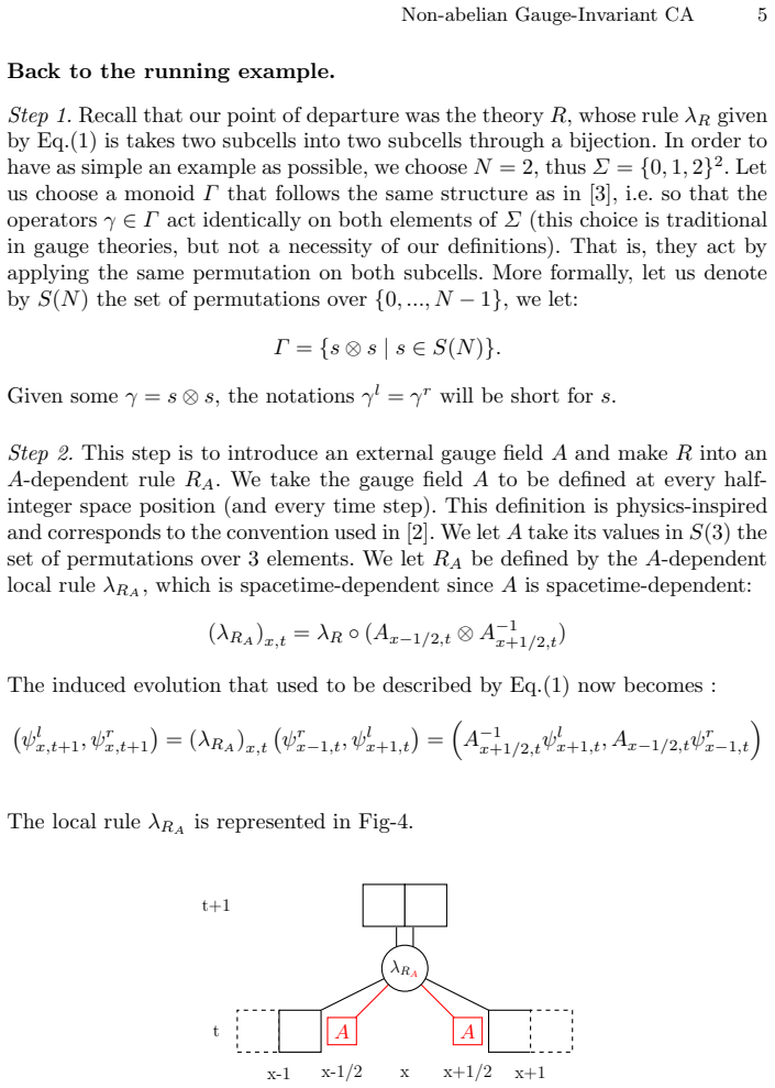
The load-bearing mechanism is the four-step gauging procedure. It starts with a CA $R$ that has no symmetry, chooses a monoid $\Gamma$ of local operators (here simultaneous permutations $s\otimes s$), and couples $R$ to a gauge field $A$ placed on half-integer edges by replacing $\lambda_R$ with $\lambda_{R_A}=\lambda_R\circ(A_{x-1/2}\otimes A_{x+1/2}^{-1})$. Imposing inhomogeneous gauge invariance fixes the transformation law $\bar{\gamma}(A)_x=\gamma^l_{x+1/2}\circ A_x\circ(\gamma^l_{x-1/2})^{-1}$, and choosing the minimal field dynamics $S_\psi=I$ produces a fully gauge-invariant $T$. The theory $Z$ that maps an input gauge transformation to the output one is taken to be the identity on $\Gamma$, which makes the invariance condition local and checkable.
What would settle it
To test the Section 3 construction, take two noncommuting permutations $s,t\in S(3)$, build a gauge transformation $\bar{\gamma}$ with $s$ at one cell and $t$ at a neighboring cell, and compare $T\circ\bar{\gamma}$ with $Z(\bar{\gamma})\circ T$ on a finite configuration; any mismatch would show the rule is not gauge-invariant. To test Proposition 4, look for a theory $T'$ that is not gauge-invariant yet satisfies condition 1 of the proposition for every configuration while failing condition 2; such an example would refute the characterization as stated.
Extended reading notes
Core claim
The paper's central construction is the cellular automaton $T$ of Section 3, with local rule $\lambda_T$ and internal state space $S(3)\times\Sigma\times S(3)$, where $\Sigma=\{0,1,2\}^2$. On a configuration the rule sends $(A_{x-1/2},\psi^l_x,\psi^r_x,A_{x+1/2})$ at time $t$ to $(A_{x-1/2},A^{-1}_{x+1/2}\psi^l_{x+1},A_{x-1/2}\psi^r_{x-1},A_{x+1/2})$ at time $t+1$. Gauge transformations act as $\gamma=s\otimes s$ with $s\in S(3)$ on $\psi$, and the gauge field transforms as $\bar{\gamma}(A)_x=\gamma^l_{x+1/2}\circ A_x\circ(\gamma^l_{x-1/2})^{-1}$; with $Z(\bar{\gamma})=\bar{\gamma}$ this yields $Z(\bar{\gamma})\circ T=T\circ\bar{\gamma}$. The paper further defines simulation and equivalence of gauge-invariant theories, characterizes them in Proposition 4, and shows that invariant sets must be formed over the joint configuration $(\psi,A)$, not over $\psi$ and $A$ separately.
Load-bearing premise
The proof of Proposition 4 moves a gauge transformation from the left of $T'$ to the right using reversibility of $Z$, and that step only works if $T'$ is itself gauge-invariant with respect to the same $Z$; the proposition does not state this assumption, so the equivalence characterization is not fully established as written.
Editorial extensions
If this is right
- If correct, the construction makes non-abelian gauge symmetry a property of a discrete reversible CA, not just of continuum field theories.
- The same four-step procedure can be applied to other base CA rules and other monoids of local operators, so the example is a template rather than an isolated case.
- The equivalence and invariant-set results give a way to say when two gauge-invariant CA are the same dynamics up to local redundancy, and they show that the gauge field cannot be factored out separately from the matter field.
- Because the gauge field is a redundancy, the dynamics of $T$ is richer than that of the original rule $R$, and the paper presents the construction as a step toward non-abelian gauge-invariant quantum cellular automata.
Reading between the lines
- The same gauging route should work for any finite group acting on the alphabet by permutations, since the derivation of Eq. (4) uses only composition and inverses; a direct check would be to instantiate the construction with a cyclic or dihedral subgroup instead of the whole symmetric group.
- The choice $S_\psi=I$ is only the minimal dynamics for the gauge field; classifying the possible inhomogeneous invariant field dynamics for a fixed $R$ would produce a family of gauge-invariant CAs and could reveal whether the choice of $S_\psi$ affects observable particle trajectories.
- Because gauge invariance makes many configurations physically equivalent, a gauge-invariant CA carries redundant encodings of the same information; that redundancy is a natural resource for fault-tolerant or error-correcting spatially distributed computation, a connection the paper lists only as future work.
Signed reviews
Editorial analysis
A structured set of objections, weighed in public.
Referee Report
Summary. The paper generalizes the authors' earlier abelian treatment of gauge-invariance in cellular automata to non-abelian symmetry groups. It reformulates gauge transformations and gauge-invariance, describes a four-step gauging procedure, and applies it to a partitioned CA with state space {0,1,2}^2 and a gauge field valued in S(3). The resulting automaton T, with local rule λT defined in Section 3, is shown to be gauge-invariant. Section 4 introduces a notion of equivalence of theories up to gauge transformations, states a characterization (Proposition 4), and discusses invariant sets of configurations.
Significance. If the Section 3 construction is correct—and it appears to be—the paper provides a concrete, explicit example showing that non-abelian gauge symmetry can be implemented in the CA framework, a useful step toward non-abelian gauge-invariant quantum cellular automata. The derivation of the gauge-field transformation law (4) from the local gauge-invariance condition is explicit and reproducible, and the final rule λT is concrete enough to check by hand. The equivalence characterization in Section 4, however, is not reliable as stated.
major comments (2)
- [Section 4, Proposition 4] Proposition 4 is false as stated: simulation of T by T′ does not imply condition 1. Let Σ={0,1}, Γ={id, flip} acting cellwise, Z(γ)=γ, T=id, and T′ be the constant-zero CA. T is gauge-invariant and Z is reversible. For every configuration c, T is simulated by T′ by taking γ=id and γ′ equal to flip on the cells where c is 1 and id elsewhere, so (γ′∘T)(c)=0=(T′∘γ)(c). But condition 1 fails for any configuration containing a 1, because T(c)=c cannot equal T′∘γ(c)=0 for any γ. This refutes the proposition in the form printed. The proof's step 'since Z is reversible, we obtain T(c)=(T′∘Z^{-1}(γ′^{-1})∘γ)(c)' implicitly requires the unstated identity Z(α)∘T′=T′∘α, i.e. gauge-invariance of T′; the counterexample shows this hypothesis is essential and absent.
- [Section 4, proof of Proposition 4] Independently of the counterexample, the proof of Proposition 4 does not align with the statement. It refers to a condition '(3)' that is not among the two listed conditions; the first bullet says '(3) implies (1) is immediate' while the second bullet 'Suppose (1)' in fact assumes the simulation condition, not condition 1. The final implication contains the line '(Z(γ3)^{-1}∘T)(c)=(T∘γ1)(c)', which should presumably read (T′∘γ1)(c), and 'implies (3)' has no stated target. These are not merely notational slips: the proposition needs to be restated with the correct hypotheses on T′ (for example, that T′ is gauge-invariant with respect to the same Z) and provided with a proof whose three implications match the stated conditions.
minor comments (3)
- [Section 3, Step 4] The sentence 'We now have an inhomogeneous gauge-invariant theory R_A, with respect to Γ and Z=I' is inconsistent with the earlier choice Z(γ)=γ and with the verification of S_ψ immediately below, which uses Z(γ)=γ; this should be corrected to avoid confusion.
- [Section 4, Invariant paragraph] The assertion that T is 'indeed equivalent' to a theory on invariant sets would benefit from a short proof or an explicit statement that it is intended as an observation, since the passage itself shows that taking quotients in the presence of a dynamical gauge field requires care.
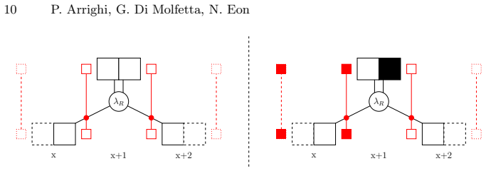
- [Figure 5 caption] The caption labels the rule as λ_R, but the figure depicts the combined theory λ_T; please correct the label for consistency with the text.
Circularity Check
No significant circularity: the Section 3 gauging construction is explicit and self-verified; only minor, non-load-bearing self-citations to the authors' prior abelian framework.
full rationale
The paper's central claim—that a non-abelian gauge-invariant CA can be constructed—is carried by the explicit calculation in Section 3. Starting from the free choice of R and Γ, Step 3 imposes the local inhomogeneous gauge-invariance condition and solves it for γ(A), obtaining Eq. (4); Step 4 checks that Sψ = I satisfies the same condition and that combining RA with Sψ yields exactly gauge-invariance condition (2). This is a self-contained derivation with no fitted constants and no prediction that is merely a renamed input. The citations to [3] and [2] supply the definitional framework, the half-integer gauge-field convention, and the common physics choice Z(γ)=γ; they are not used as unexamined theorems that force the non-abelian result. The only notable defect is in Proposition 4: the proof step "since Z is reversible, we obtain T(c) = (T′ ∘ Z^{-1}(γ′^{-1}) ∘ γ)(c)" silently requires T′ to be gauge-invariant with respect to the same Z, which is not assumed; this is a correctness gap in the equivalence characterization, but it is not a circular reduction of the paper's central construction to its inputs. Accordingly no specific circular step is identified.
Assumptions & free parameters
assumptions (4)
- domain assumption Gauge transformations form a group (or monoid) acting pointwise on configurations; Γ^Z is the set of such transformations.
- domain assumption The theory R is a reversible cellular automaton expressible in block-circuit (Margolus) form.
- domain assumption The theory Z is deterministic and reversible.
- ad hoc to paper The simulated theory T' is gauge-invariant with respect to the same Z (unstated).
invented entities (1)
-
Gauge field A valued in S(3) at half-integer sites
Cite this review
Pith. "Pith review of Non-Abelian Gauge-Invariant Cellular Automata." pith.science (2026). https://pith.science/paper/4SRHGPGH
@misc{pith2026190801229,
  author       = {Pith},
  title        = {Pith review of: Non-Abelian Gauge-Invariant Cellular Automata},
  year         = {2026},
  howpublished = {\url{https://pith.science/paper/4SRHGPGH}},
  note         = {Machine review of arXiv:1908.01229}
}
read the original abstract
Gauge-invariance is a mathematical concept that has profound implications in Physics---as it provides the justification of the fundamental interactions. It was recently adapted to the Cellular Automaton (CA) framework, in a restricted case. In this paper, this treatment is generalized to non-abelian gauge-invariance, including the notions of gauge-equivalent theories and gauge-invariants of configurations
Figures


Figures from the paper (3 more)


Reference graph
Works this paper leans on
-
[1]
Physical Review A 94(1), 012335 (2016)
Arnault, P., Di Molfetta, G., Brachet, M., Debbasch, F.: Quantum walks and non-abelian discrete gauge theory. Physical Review A 94(1), 012335 (2016)
work page 2016
-
[2]
arXiv preprint arXiv:1903.07007 (2019)
Arrighi, P., B \'e ny, C., Farrelly, T.: A quantum cellular automaton for one-dimensional qed. arXiv preprint arXiv:1903.07007 (2019)
arXiv 2019
-
[3]
In: International Workshop on Cellular Automata and Discrete Complex Systems
Arrighi, P., Di Molfetta, G., Eon, N.: A gauge-invariant reversible cellular automaton. In: International Workshop on Cellular Automata and Discrete Complex Systems. pp. 1--12. Springer (2018)
work page 2018
-
[4]
Annals of Physics 303(1), 2--30 (2003)
Kitaev, A.Y.: Fault-tolerant quantum computation by anyons. Annals of Physics 303(1), 2--30 (2003)
work page 2003
-
[5]
Reviews of Modern Physics 80(3), 1083 (2008)
Nayak, C., Simon, S.H., Stern, A., Freedman, M., Sarma, S.D.: Non-abelian anyons and topological quantum computation. Reviews of Modern Physics 80(3), 1083 (2008)
work page 2008
-
[6]
Princeton University Press (2013)
Quigg, C.: Gauge theories of the strong, weak, and electromagnetic interactions. Princeton University Press (2013)
work page 2013
-
[7]
Lecture Notes in Computer Science p
Salo, V., Törmä, I.: Color blind cellular automata. Lecture Notes in Computer Science p. 139–154 (2013)
work page 2013
-
[8]
MIT Press, Cambridge MA (1987)
Toffoli, T., Margolus, N.: Cellular Automata Machine -- A new Environment for Modelling . MIT Press, Cambridge MA (1987)
work page 1987
Show all 13 references
-
[9]
Topics in Contemporary Probability and Its Applications pp
Toom, A.: Cellular automata with errors: Problems for students of probability . Topics in Contemporary Probability and Its Applications pp. 117--157 (1995)
1995
-
[10]
Stochastic Cellular Systems: ergodicity, memory, morphogenesis
Toom, A., Vasilyev, N., Stavskaya, O., Mityushin, L., Kurdyumov, G., Pirogov, S.: Discrete Local Markov Systems. Stochastic Cellular Systems: ergodicity, memory, morphogenesis. Ed. by R. Dobrushin, V. Kryukov and A. Toom. Nonlinear Science: theory and applications (1990)
1990
-
[11]
Springer (2004)
Wolf-Gladrow, D.A.: Lattice-gas cellular automata and lattice Boltzmann models: an introduction. Springer (2004)
2004
-
[12]
, " * write output.state after.block = add.period write
ENTRY address author booktitle chapter doi edition editor eid howpublished institution journal key month note number organization pages publisher school series title type url volume year label INTEGERS output.state before.all mid.sentence after.sentence after.block FUNCTION in...
-
[13]
write newline
" write newline "" before.all 'output.state := FUNCTION n.dashify 't := "" t empty not t #1 #1 substring "-" = t #1 #2 substring "--" = not "--" * t #2 global.max substring 't := t #1 #1 substring "-" = "-" * t #2 global.max substring 't := while if t #1 #1 substring * t #2 gl...
Reviewed August 14, 2026 · model on record in the stance chip above.
Discussion (0). Continue with ORCID to comment.