REVIEW 3 major objections 5 minor 64 references
Deep regularization networks for inverse problems with noisy operators
T0 review · 3 major / 5 minor · reviewed 2026-08-07 · deepseek-v4-flash
Pith's one-line read A two-step neural network learns regularization maps for inverse problems with noisy operators and improves image contrast.
desk verdict A worthwhile two-step learning idea for noisy-operator regularization, but the Step 2 quality gains are carried by early stopping, not by the stated objective. read the letter →
The pith
A machine-rendered reading of the paper's core claim, the machinery that carries it, and where it could break.
The reading
What carries the argument
The load-bearing object is the regularization network (R-Net), an MLP whose input is the right-hand side pattern projected onto the left singular vectors of the noisy scattering operator, $U^*u_L$, and whose output is a Tikhonov parameter $\alpha_{NN}$ for that pattern. The spectral filter factors $D_{jj}/(\alpha_{NN}+D_{jj}^2)$ then define the regularized solution $g_{NN}=VD^\dagger U^*u_L$, which is what the linear sampling method indicator uses. The argument is carried by two training mechanisms: (1) in Step 1, the informed loss combines a normalized misfit to the Morozov $\alpha_M$ with the squared Morozov discrepancy functional $J_2^t$ evaluated at a rough threshold $\eta_\circ$, and the chosen weights in (19) make both gradient terms $O(\partial \alpha_{NN}/\partial w)$, so the discrepancy logic is learned without an inner optimization for loss balancing; (2) in Step 2, minimizing $J_{img}$ tailors $\alpha$ toward a min-norm solution, and Algorithm 2 stops training when the rms of normalized training or validation loss variations crosses a threshold or their ratio leaves an interval, which is the mechanism claimed to convert extra training into higher image contrast without overfitting.
What would settle it
In the 25-percent-noise cases, re-run Step 2 with the stopping thresholds $\sigma_a$ and $\sigma_r$ removed so training continues for many more epochs, and record the defect-to-background contrast at every epoch: if contrast keeps improving after the rule would have stopped, or never peaks near the rule's stop point, then the image enhancement is not produced by the loss-trajectory regulation that carries the claim.
Extended reading notes
Core claim
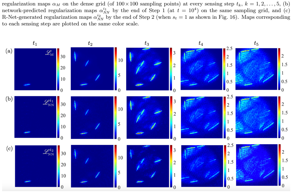
The central discovery claimed is that a network trained first to imitate cheap, low-resolution Morozov discrepancy maps and then fine-tuned on the Tikhonov imaging loss can produce linear sampling method reconstructions whose contrast matches or beats the Morozov maps obtained by per-time-step manual tuning, even when the scattering operator carries 25 percent noise. The network takes the projected right-hand side $U^*u_L$ as input and outputs the Tikhonov parameter $\alpha$; with that $\alpha$ the spectral filter factors $D_{jj}/(\alpha + D_{jj}^2)$ supply the regularized solution. Step 1 uses an informed loss that includes the discrepancy principle itself, with adaptive weights that normalize the gradients without a second optimization loop, and Step 2 minimizes the Bayes-risk Tikhonov loss with an early-stopping rule based on normalized training-versus-validation loss trajectories. The evidence is a synthetic elastic-plate experiment in which a single crack grows into a cloud of fifteen cracks over five sensing steps; at 25 percent noise the Step-2 images show higher defect-to-background contrast than the manually tuned Morozov baseline at almost every sensing step.
Load-bearing premise
The paper's claimed contrast gain in Step 2 rests on a heuristic early-stopping rule: the relative trajectories of training and validation Tikhonov losses are assumed to reveal when further minimization stops helping the image, and if that rule fails on a new geometry or noise level, the refinement step can make reconstructions worse rather than better.
Editorial extensions
If this is right
- Dense regularization maps for the full 100 by 100 search grid can be produced from a network trained on only 2,500 of 720,000 right-hand side patterns.
- A discrepancy-informed Step 1 generalizes better than direct regression on Morozov maps, so the choice of training loss determines whether the network can be refined in Step 2.
- Step 2 improves the mean and maximum contrast of LSM images relative to manually tuned Morozov reconstructions, with the largest gains appearing at 25 percent noise and late sensing steps.
- Because Step 2 needs no labeled optimal regularization maps, the network can adapt to test data online, removing the need to tune the Morozov threshold by hand.
Reading between the lines
- Extension: Apply the same scheme to generalized linear sampling method or time-domain imaging, where per-pattern root-finding is even more expensive; the discrepancy functional changes but the projection-plus-early-stopping logic should transfer, and this is untested in the paper.
- Extension: The only guard against $\alpha$ collapsing toward zero in Step 2 is the stopping rule, so a deployment should monitor a ground-truth-free contrast metric alongside the loss trajectories; the paper reports no correlation analysis between loss rms and contrast.
- Extension: If low-resolution-to-dense generalization is the mechanism, substituting a resolution-independent network for the fixed-size MLP could let one trained model serve arbitrarily fine grids, which the paper flags as possible but does not demonstrate.
Editorial analysis
A structured set of objections, weighed in public.
Referee Report
Summary. The paper proposes a two-step deep-learning method for choosing per-right-hand-side Tikhonov parameters in linear sampling method (LSM) reconstructions when the scattering operator itself is noisy. In Step 1, an MLP is trained on low-resolution regularization maps produced by the Morozov discrepancy principle with a rough threshold η0; two modes are considered, a basic squared-error mode and a 'discrepancy-informed' mode that adds the discrepancy functional to the loss with adaptive weights. In Step 2, the network is fine-tuned by minimizing the Tikhonov imaging loss on the training right-hand sides, with an early-stopping rule based on training and validation loss trajectories. The method is tested on synthetic elastodynamic data for a plate with an evolving damage zone at 0%, 10%, and 25% noise, and the resulting LSM images are compared with manually tuned Morozov reconstructions through contrast metrics. The authors report that discrepancy-informed R-Nets generalize from 50×50 to 100×100 grids and that Step 2 increases contrast, especially at high noise.
Significance. The engineering problem is relevant: per-RHS Tikhonov regularization for LSM is a genuine bottleneck for real-time imaging, and the idea of learning a map from projected right-hand sides to α from coarse Morozov maps is attractive. The paper's strengths include complete algorithmic pseudocode, an explicit SVD-based architecture, a substantial synthetic testbed with five damage configurations and three noise levels, and an honest comparison with manually tuned Morozov baselines. If the Step-2 claim were supported, the practical contribution would be valuable. However, the current manuscript does not establish that Step 2 improves images as a consequence of the stated objective; the objective is degenerate in α, and the claimed gains appear to be selected by early-stopping thresholds. The discrepancy-functional equations also contain an internal inconsistency that affects the Step-1 labels and the loss-balancing derivation.
major comments (3)
- [3.2, Eqs. (22)–(24)] The Step 2 objective is degenerate in α and does not, as stated, drive the network toward higher-quality images. For a fixed right-hand side u_L, substituting (23) into (22) gives J_t(α)=Σ_j α |(u_j^*,u_L)|^2/(α+d_j^2), which is strictly increasing for α>0 and tends to 0 as α→0; the unconstrained minimization therefore pushes α_NN toward 0 and ||g_NN|| toward infinity, and no interior optimum exists. Because V_img in (24) is the same functional evaluated on a validation set, its trajectory cannot independently detect this norm blow-up. As written, the reported Step 2 contrast gains are selected by the particular thresholds σ_r=5, σ_a=10^{-4}, N_rms=10^4 and the learning rate 5×10^{-8}, not by a proven property of the objective. Please either add a penalty or constraint that gives (22) a nontrivial minimizer, or reframe Step 2 as an empirically early-stopped heuristic and provide a sensitivity analysis over these thresholds plus an independent quality measure on held-out configurations.
- [3.1.2 and 4.4, Eqs. (15), (19), (32)] The discrepancy functional is internally inconsistent. For the Tikhonov filter in (23), the Morozov condition ||F^δ g−u_L||=η||g|| is Σ_j (α²−η²D_jj²)/(α+D_jj²)² |(u_j^*,u_L)|²=0, but Eqs. (15) and (32) write the numerator as α−η²D_jj². The derivative in (19), 2D_jj²(α+η²)/(α+D_jj²)³, is the derivative of the α² version, not of the printed α version. This matters because (32) generates the Morozov labels used for Step 1 training and for the manually tuned baselines, while (19) is the basis of the proposed loss-balancing weights. The equations should be reconciled and the numerical results re-checked with the corrected Morozov functional.
- [4.4, Figs. 18, 22, 26 and Tables 4–6] The evaluation of Step 2 is transductive: the network is trained on a subset of the RHS patterns of the same damage configuration, and the reported LSM images are then reconstructed from the full RHS dictionary of that same configuration, including the patterns used in Step 2. The claimed 'remarkable enhancement' therefore does not yet demonstrate generalization to unseen configurations. Please report results on a genuinely held-out configuration, or at least on RHS patterns excluded from both training steps, and state whether the contrast gains persist there.
minor comments (5)
- [Eq. (24)] The summation upper limit is written as Ntrn, although the validation set is indexed by ν=1,…,Nν; this should be Nν.
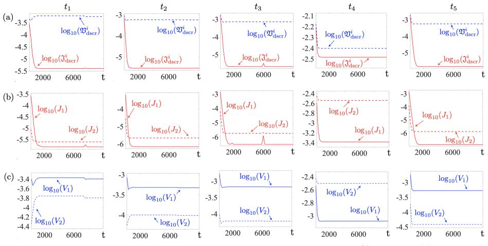
- [4.4, informed R-Net Step 1] The text states that the training runs for t∈[1,1000], while Step 2 is said to start at t=10001 and the caption of Fig. 17 says Step 1 ends at t=10^4; please reconcile the epoch counts.
- [3.2, sentence after Eq. (23)] The statement that minimizing (22) 'minimizes the residual ... while maximizing the LSM indicator functional' is not a direct consequence of the displayed objective, since it trades residual against ||g||² and does not explicitly maximize 1/||g||; please rephrase.
- [Algorithm 2] The stopping rule uses OR conditions, so a flattening of either the training or the validation loss can stop training; a patience parameter or a more explicit combination of the conditions may better match the stated goal of detecting overfitting.
- [Table 7] Reporting the time per epoch is useful, but the total wall-clock time until the stopping criterion is met, including the validation-loss evaluation in Step 2, would better support the real-time imaging claim.
Circularity Check
Step 2 'enhancement' reduces to a stopping-time artifact: the Tikhonov loss (22) with g_NN from (23) is strictly increasing in alpha and vanishes at alpha->0, so no interior optimum exists and reported gains are selected by Algorithm 2 thresholds, not by the stated imaging objective.
-
self definitional
[Section 3.2, Eqs. (22)-(23), Algorithm 2, and Section 4.4 around Eq. (34)]
"In this step, the learning objective is to furnish regularization maps {αtNN}t=1,2,...,Ntrn that optimize the imaging (i.e., Tikhonov) loss function within the Bayes risk minimization framework, Jimg = ... wherein ∀t ∈ 1,2,...,Ntrn, gtNN(αtNN) = V D†U∗utL, D†(D, αtNN) = diag { Djj/(αtNN + D2jj) }."
Substituting Eq. (23) into Eq. (22) gives, per RHS pattern, Jimg(α) = Σ_j α |(u_j*,u_L)|^2 / (α + d_j^2) with d_j = D_jj. This is strictly increasing for α > 0 and tends to 0 as α → 0, so the unconstrained minimum of the Step-2 objective is at α → 0, where ||g_NN|| diverges and the LSM indicator 1/||g|| collapses. Hence the claimed 'optimization' cannot select an interior regularizer or enhance contrast; every finite-α result is effectively chosen by the early-stopping thresholds in Algorithm 2 (σ_r = 5, σ_a = 10^-4, N_rms = 10000). The derivation 'minimizing the imaging loss improves the image' reduces by construction to 'a chosen stopping time selects the image', so the enhancement claim is not independently derived from the objective.
-
fitted input called prediction
[Abstract and Section 3.2, Eqs. (22)-(24), with results in Tables 4-6]
"This approach enables direct learning from test data and dispenses with the need for a-priori knowledge of the optimal regularization maps (or labeled datasets) for training."
Step 2 optimizes the network on a subset {U∗ut_L} of the same right-hand-side library {U∗un_L} that also defines the validation set and the final LSM reconstructions, with the validation set being the complement of the training subset within that same library. The reported contrast gains in Tables 4-6 are therefore measured on the very data distribution used to fit the Step-2 parameters, so the 'enhancement' is partly a measure of fitting to the evaluation data rather than an independent prediction. The paper explicitly advertises learning from 'test data' as an advantage, which makes the quality claim self-referential rather than externally validated.
full rationale
Step 1 is a legitimate supervised learning stage: low-resolution Morozov maps provide an independent anchor, and validation is performed on held-out RHS patterns. The self-citations to [41,42] establish operator properties and [47] only inspires loss balancing; none of these are load-bearing for the central claim. The circularity is concentrated in Step 2. Its Tikhonov objective is degenerate: because g_NN(α) is by construction the minimizer of the same loss, substituting it into Eq. (22) yields a function that is minimized at α → 0, so no finite interior optimum exists. The advertised 'optimization' therefore cannot be the mechanism of contrast enhancement; the reported images are selected by Algorithm 2's manually fixed stopping thresholds. In addition, the evaluation is performed on the same RHS library from which the Step-2 training and validation sets are drawn, so the headline claim of 'remarkable enhancement' rests on a partly self-referential fitting loop. Step 1 provides independent content, but the Step-2 'prediction' reduces by construction to the stopping rule and to fitting the evaluation library, giving a partial circularity score of 6.
Assumptions & free parameters
free parameters (4)
- Morozov threshold η◦ for training labels =
0.3 (recommended interval [0.3,0.5))
- Manually tuned baseline thresholds η_k^{np} =
0.08 to 0.30 depending on time step and noise level (Table 2)
- Network training hyperparameters =
learning rates 1e-5, 5e-6, 5e-8; epochs up to 10000; stop thresholds σa=1e-4, σr=5; Nrms=10000
- Downsampling factor and training grid size =
m=2, 50x50 training grid, Ntrn=2500
assumptions (7)
- domain assumption The scattering operator F^δ is compact, injective, and has dense range.
- domain assumption Classical LSM with B=I is an adequate imaging model; generalized LSM forms are deferred.
- domain assumption Noise acts multiplicatively as Fδ=(I+Nδ)F with entries uniformly distributed in [-δ,δ].
- ad hoc to paper One trial scatterer per sampling point, selected by min-norm (Eq 10), and a 50x50 grid are representative for training the regularization map.
- ad hoc to paper Minimizing the Tikhonov loss in Step 2 improves LSM image contrast.
- ad hoc to paper The validation-loss trajectory criterion (Algorithm 2) detects overfitting and preserves image quality.
- standard math MLP with two ReLU hidden layers is sufficient to represent the regularization map.
Cite this review
Pith. "Pith review of Deep regularization networks for inverse problems with noisy operators." pith.science (2026). https://pith.science/paper/4WJO4EIC
@misc{pith2026250607008,
  author       = {Pith},
  title        = {Pith review of: Deep regularization networks for inverse problems with noisy operators},
  year         = {2026},
  howpublished = {\url{https://pith.science/paper/4WJO4EIC}},
  note         = {Machine review of arXiv:2506.07008}
}
read the original abstract
A supervised learning approach is proposed for regularization of large inverse problems where the main operator is built from noisy data. This is germane to superresolution imaging via the sampling indicators of the inverse scattering theory. We aim to accelerate the spatiotemporal regularization process for this class of inverse problems to enable real-time imaging. In this approach, a neural operator maps each pattern on the right-hand side of the scattering equation to its affiliated regularization parameter. The network is trained in two steps which entails: (1) training on low-resolution regularization maps furnished by the Morozov discrepancy principle with nonoptimal thresholds, and (2) optimizing network predictions through minimization of the Tikhonov loss function regulated by the validation loss. Step 2 allows for tailoring of the approximate maps of Step 1 toward construction of higher quality images. This approach enables direct learning from test data and dispenses with the need for a-priori knowledge of the optimal regularization maps. The network, trained on low-resolution data, quickly generates dense regularization maps for high-resolution imaging. We highlight the importance of the training loss function on the network's generalizability. In particular, we demonstrate that networks informed by the logic of discrepancy principle lead to images of higher contrast. In this case, the training process involves many-objective optimization. We propose a new method to adaptively select the appropriate loss weights during training without requiring an additional optimization process. The proposed approach is synthetically examined for imaging damage evolution in an elastic plate. The results indicate that the discrepancy-informed regularization networks not only accelerate the imaging process, but also remarkably enhance the image quality in complex environments.
Figures


Figures from the paper (23 more)






Reference graph
Works this paper leans on
-
[1]
V. Narumanchi, F. Pourahmadian, J. Lum, A. Townsend, J. W. Tringe, D. M. Stobbe, T. W. Murray, Laser ultrasonic imaging of subsurface defects with the linear sampling method, Optics express 31 (5) (2023) 9098–9111. doi:10.1364/OE.485084
-
[2]
F. Pourahmadian, H. Yue, Laboratory application of sampling approaches to inverse scattering, Inverse Problems 37 (5) (2021) 055012. doi:10.1088/1361-6420/abf161
- [3]
-
[4]
P. Monk, M. Pena, V. Selgas, Multifrequency linear sampling method on experimental datasets, IEEE Transactions on Antennas and Propagation 71 (11) (2023) 8788–8798. doi:10.1109/TAP. 2023.3298974
arXiv 2023
-
[5]
Recoquillay, On the use of phase laws for the linear sampling method in an elastic waveg- uide
A. Recoquillay, On the use of phase laws for the linear sampling method in an elastic waveg- uide. application to nondestructive testing, Wave Motion 133 (2025) 103447. doi:10.1016/j. wavemoti.2024.103447
arXiv 2025
- [6]
- [7]
- [8]
Show all 64 references
-
[9]
Taheri, Nondestructive evaluation and in-situ monitoring for metal additive manufacturing, Ph.D
H. Taheri, Nondestructive evaluation and in-situ monitoring for metal additive manufacturing, Ph.D. thesis, Iowa State University (2018). doi:10.1063/1.5031503
2018 doi
-
[10]
Haber, L
E. Haber, L. Tenorio, Learning regularization functionals?a supervised training approach, In- verse Problems 19 (3) (2003) 611. doi:10.1088/0266-5611/19/3/309
2003 doi
-
[11]
Habring, M
A. Habring, M. Holler, Neural-network-based regularization methods for inverse problems in imaging, GAMM-Mitteilungen 47 (4) (2024) e202470004. doi:10.1002/gamm.202470004
2024 doi
-
[12]
Arridge, P
S. Arridge, P. Maass, O. ¨Oktem, C.-B. Sch ¨onlieb, Solving inverse problems using data-driven models, Acta Numerica 28 (2019) 1–174. doi:10.1017/s0962492919000059
2019 doi
-
[13]
B. M. Afkham, J. Chung, M. Chung, Learning regularization parameters of inverse problems via deep neural networks, Inverse Problems 37 (10) (2021) 105017. doi:10.1088/1361-6420/ ac245d
2021 doi
-
[14]
H. Li, J. Schwab, S. Antholzer, M. Haltmeier, Nett: Solving inverse problems with deep neural networks, Inverse Problems 36 (6) (2020) 065005. doi:10.1088/1361-6420/ab6d57
2020 doi
-
[15]
Hauptmann, S
A. Hauptmann, S. Mukherjee, C.-B. Sch ¨onlieb, F. Sherry, Convergent regularization in inverse problems and linear plug-and-play denoisers, Foundations of Computational Mathematics (2024) 1–34doi:10.1007/s10208-024-09654-x
2024 doi
-
[16]
Santambrogio, M
C. Santambrogio, M. Pragliola, A. Lanza, M. Donatelli, L. Calatroni, Whiteness-based bilevel learning of regularization parameters in imaging, in: 2024 32nd European Signal Processing Conference (EUSIPCO), IEEE, 2024, pp. 1801–1805. doi:10.23919/eusipco63174.2024. 10715121
2024
-
[17]
A. N. Tikhonov, Solution of incorrectly formulated problems and the regularization method., Sov Dok 4 (1963) 1035–1038. doi:10.1016/0041-5553(63)90137-x
1963 doi
-
[18]
Kress, Linear integral equation, Springer, Berlin, 1999
R. Kress, Linear integral equation, Springer, Berlin, 1999. doi:10.1007/978-1-4612-0559-3
1999 doi
-
[19]
V. A. Morozov, M. Stessin, Regularization methods for ill-posed problems, CRC Press, 1993. doi:10.1007/bf00861942
1993 doi
-
[20]
P. C. Hansen, Discrete inverse problems: insight and algorithms, SIAM, 2010. doi:10.1137/ 1.9780898718836
2010
-
[21]
P. C. Hansen, D. P. O’Leary, The use of the l-curve in the regularization of discrete ill-posed prob- lems, SIAM journal on scientific computing 14 (6) (1993) 1487–1503. doi:10.1137/0914086
1993 doi
-
[22]
Y. Xu, F. Pourahmadian, J. Song, C. Wang, Deep learning for full-field ultrasonic characteri- zation, Mechanical Systems and Signal Processing 201 (2023) 110668. doi:10.1016/j.ymssp. 2023.110668. 35
2023
-
[23]
Kaltenbacher, A
B. Kaltenbacher, A. Neubauer, O. Scherzer, Iterative regularization methods for nonlinear ill- posed problems, Walter de Gruyter, 2008. doi:10.1515/9783110208276
2008 doi
-
[24]
Benning, M
M. Benning, M. Burger, Modern regularization methods for inverse problems, Acta numerica 27 (2018) 1–111. doi:10.1017/s0962492918000016
2018 doi
-
[25]
N. P. Galatsanos, A. K. Katsaggelos, Methods for choosing the regularization parameter and estimating the noise variance in image restoration and their relation, IEEE Transactions on image processing 1 (3) (1992) 322–336. doi:10.1109/83.148606
1992 doi
-
[26]
C. R. Vogel, Non-convergence of the l-curve regularization parameter selection method, Inverse problems 12 (4) (1996) 535. doi:10.1088/0266-5611/12/4/013
1996 doi
-
[27]
J. L. Mead, R. A. Renaut, A newton root-finding algorithm for estimating the regularization parameter for solving ill-conditioned least squares problems, Inverse Problems 25 (2) (2008) 025002. doi:10.1088/0266-5611/25/2/025002
2008 doi
-
[28]
Haber, L
E. Haber, L. Horesh, L. Tenorio, Numerical methods for experimental design of large-scale linear ill-posed inverse problems, Inverse Problems 24 (5) (2008) 055012. doi:10.1088/0266-5611/ 24/5/055012
2008 doi
-
[29]
Chung, S
J. Chung, S. Gazzola, Computational methods for large-scale inverse problems: a survey on hybrid projection methods, Siam Review 66 (2) (2024) 205–284. doi:10.1137/21m1441420
2024 doi
-
[30]
Goujon, S
A. Goujon, S. Neumayer, P. Bohra, S. Ducotterd, M. Unser, A neural-network-based convex regularizer for inverse problems, IEEE Transactions on Computational Imaging 9 (2023) 781–
2023
-
[31]
Kofler, F
A. Kofler, F. Altekr ¨uger, F. Antarou Ba, C. Kolbitsch, E. Papoutsellis, D. Schote, C. Sirotenko, F. F. Zimmermann, K. Papafitsoros, Learning regularization parameter-maps for variational image reconstruction using deep neural networks and algorithm unrolling, SIAM Journal on...
2023 doi
-
[32]
Eliasof, E
M. Eliasof, E. Haber, E. Treister, Drip: deep regularizers for inverse problems, Inverse Problems 40 (1) (2023) 015006. doi:10.1088/1361-6420/ad0f3b
2023 doi
-
[33]
Antil, Z
H. Antil, Z. W. Di, R. Khatri, Bilevel optimization, deep learning and fractional laplacian regularization with applications in tomography, Inverse Problems 36 (6) (2020) 064001. doi: 10.1088/1361-6420/ab80d7
2020 doi
-
[34]
S. Lunz, O. ¨Oktem, C.-B. Sch ¨onlieb, Adversarial regularizers in inverse problems, Advances in neural information processing systems 31 (2018). doi:10.1109/icassp48485.2024.10447719
2018
-
[35]
Calatroni, C
L. Calatroni, C. Cao, J. C. De Los Reyes, C.-B. Sch ¨onlieb, T. Valkonen, Bilevel approaches for learning of variational imaging models, Variational Methods: In Imaging and Geometric Control 18 (252) (2017) 2. doi:10.1515/9783110430394-008
2017 doi
-
[36]
Chung, M
J. Chung, M. I. Espa˜ nol, Learning regularization parameters for general-form tikhonov, Inverse Problems 33 (7) (2017) 074004. doi:10.1088/1361-6420/33/7/074004
2017 doi
-
[37]
Chung, M
J. Chung, M. Chung, D. P. O’Leary, Designing optimal spectral filters for inverse problems, SIAM Journal on Scientific Computing 33 (6) (2011) 3132–3152. doi:10.1137/100812938. 36
2011 doi
-
[38]
Cakoni, D
F. Cakoni, D. Colton, P. Monk, The linear sampling method in inverse electromagnetic scatter- ing, SIAM, 2011. doi:10.1137/1.9780898719406
2011 doi
-
[39]
Colton, H
D. Colton, H. Haddar, M. Piana, The linear sampling method in inverse electromagnetic scat- tering theory, Inverse problems 19 (6) (2003) S105. doi:10.1088/0266-5611/19/6/057
2003 doi
-
[40]
Audibert, H
L. Audibert, H. Haddar, A generalized formulation of the linear sampling method with exact characterization of targets in terms of farfield measurements, Inverse Problems 30 (2014) 035011. doi:10.1088/0266-5611/30/3/035011
2014 doi
-
[41]
Pourahmadian, B
F. Pourahmadian, B. B. Guzina, H. Haddar, Generalized linear sampling method for elastic- wave sensing of heterogeneous fractures, Inverse Problems 33 (5) (2017) 055007. doi:10.1088/ 1361-6420/33/5/055007
2017
-
[42]
Pourahmadian, H
F. Pourahmadian, H. Haddar, Differential tomography of micromechanical evolution in elastic materials of unknown micro/macrostructure, SIAM Journal on Imaging Sciences 13 (3) (2020) 1302–1330. doi:10.1137/19m1305707
2020 doi
-
[43]
V. A. Morozov, Methods for solving incorrectly posed problems, Springer Science & Business Media, 2012. doi:10.1109/uwbusis.2012.6379801
2012
-
[44]
Kirsch, An introduction to the mathematical theory of inverse problems, Vol
A. Kirsch, An introduction to the mathematical theory of inverse problems, Vol. 120, Springer,
-
[45]
H. W. Engl, M. Hanke, A. Neubauer, Regularization of inverse problems, Vol. 375, Springer Science & Business Media, 1996. doi:10.1007/978-94-009-1740-8
1996 doi
-
[46]
Z. Chen, V. Badrinarayanan, C.-Y. Lee, A. Rabinovich, Gradnorm: gradient normalization for adaptive loss balancing in deep multitask networks, in: Proceedings of the 35th In- ternational Conference on Machine Learning, PMLR, 2018, pp. 794–803. doi:10.1016/ b978-0-12-813677-5.00003-1
2018
-
[47]
Y. Xu, F. Pourahmadian, Network scaling and scale-driven loss balancing for intelligent char- acterization of poroelastic systems, Journal of Computational Physics 537 (2025) 114129. doi:10.1016/j.jcp.2025.114129
2025
-
[48]
Audibert, H
L. Audibert, H. Haddar, The generalized linear sampling method for limited aperture measure- ments, SIAM Journal on Imaging Sciences 10 (2) (2017) 845–870. doi:10.1137/16m110112x
2017 doi
-
[49]
Hornik, M
K. Hornik, M. Stinchcombe, H. White, Multilayer feedforward networks are universal approxi- mators, Neural networks 2 (5) (1989) 359–366. doi:10.1016/0893-6080(89)90020-8
1989 doi
-
[50]
Z. Li, N. Kovachki, K. Azizzadenesheli, B. Liu, K. Bhattacharya, A. Stuart, A. Anand- kumar, Fourier neural operator for parametric partial differential equations, arXiv preprint arXiv:2010.08895 (2020). doi:10.1142/12052
2020 arXiv
-
[51]
Kovachki, S
N. Kovachki, S. Lanthaler, S. Mishra, On universal approximation and error bounds for fourier neural operators, The Journal of Machine Learning Research 22 (1) (2021) 13237–13312. doi: 10.5802/smai-jcm.74. 37
2021 doi
-
[52]
H. You, Q. Zhang, C. J. Ross, C.-H. Lee, Y. Yu, Learning deep implicit fourier neural operators (ifnos) with applications to heterogeneous material modeling, Computer Methods in Applied Mechanics and Engineering 398 (2022) 115296. doi:10.1016/j.cma.2022.115296
2022
-
[53]
A. A. Heydari, C. A. Thompson, A. Mehmood, Softadapt: Techniques for adaptive loss weighting of neural networks with multi-part loss functions, arXiv preprint arXiv:1912.12355 (2019). doi: 10.1080/0022250x.2019.1694519
2019 arXiv
-
[54]
Kendall, Y
A. Kendall, Y. Gal, R. Cipolla, Multi-task learning using uncertainty to weigh losses for scene geometry and semantics, in: Proceedings of the IEEE Conference on Computer Vision and Pattern Recognition, 2017, pp. 7482–7491. doi:10.5244/c.31.57
2017 doi
-
[55]
S. Wang, Y. Teng, P. Perdikaris, Understanding and mitigating gradient flow pathologies in physics-informed neural networks, SIAM Journal on Scientific Computing 43 (5) (2021) A3055– A3081. doi:10.1137/20m1318043
2021 doi
-
[56]
Bischof, M
R. Bischof, M. Kraus, Multi-objective loss balancing for physics-informed deep learning, arXiv preprint arXiv:2110.09813 (2021). doi:10.3390/socsci10100389
2021
-
[57]
Bonnet, Boundary integral equations methods for solids and fluids, Wiley, 1999
M. Bonnet, Boundary integral equations methods for solids and fluids, Wiley, 1999. doi: 10.1023/a:1004795120236
1999 doi
-
[58]
Avatavului, M
C. Avatavului, M. Prodan, Evaluating image contrast: a comprehensive review and comparison of metrics, Journal of Information Systems & Operations Management 17 (1) (2023) 143–160. doi:10.1109/iciip.2011.6108900
2023
-
[59]
Otsu, A threshold selection method from gray-level histograms, Automatica 11 (285-296) (1975) 23–27
N. Otsu, A threshold selection method from gray-level histograms, Automatica 11 (285-296) (1975) 23–27. doi:10.3724/sp.j.1004.2009.01022
1975 arXiv
-
[60]
Zhang, G
Z. Zhang, G. Dai, X. Liang, S. Yu, L. Li, Y. Xie, Can signal-to-noise ratio perform as a baseline indicator for medical image quality assessment, IEEE Access 6 (2018) 11534–11543. doi:10. 1109/access.2018.2796632
2018
-
[61]
T. L. Szabo, Diagnostic ultrasound imaging: inside out, Academic press, 2013. doi:10.7863/ jum.2013.32.4.573. 38
2013
-
[795]
doi:10.1109/tci.2023.3306100
2023
-
[2011]
doi:10.1007/978-1-4419-8474-6
-
[2022]
doi:10.1137/1.9781611977424
Reviewed August 7, 2026 · model on record in the stance chip above.
Discussion (0). Sign in to comment.