A Modified Moving Reference Frame Method for Propeller Resolution

Antonios Kritikos; Denis Andreev; Georgios Bletsos; Niklas K\"uhl; Thomas Rung

REVIEW 3 major objections 6 minor 2 references

A Modified Moving Reference Frame Method for Propeller Resolution

T0 review · 3 major / 6 minor · reviewed 2026-08-15 · deepseek-v4-flash

Challenge this review Re-run · record.json Download PDF Read on arXiv ↗ Review JSON

Pith's one-line read A smoothed reference frame removed the velocity jump at propeller-domain interfaces in ship CFD.

desk verdict Clean derivation and solid integral validation, but the local-accuracy payoff is calibrated rather than independently tested. read the letter →

arxiv 2607.24630 v1 pith:4XXV6U6J submitted 2026-07-27 physics.flu-dyn physics.comp-ph

Denis Andreev , Georgios Bletsos , Antonios Kritikos , Niklas Kühl , Thomas Rung This is my paper · ORCID

classification physics.flu-dynphysics.comp-ph

keywords movingreferenceframepartiallyrotatinggridpropeller-hullinteractionself-propulsionsimulationJapanBulkCarrierRANSslidinginterfacecontinuity

verification ladder T0 review T1 audit T2 compute T3 formal

The pith

A machine-rendered reading of the paper's core claim, the machinery that carries it, and where it could break.

The reading

This paper tries to establish that a moving reference frame (MRF) whose rotation rate is spatially damped to zero at the domain boundary can replace the abrupt rotating-stationary interface of classical MRF and restore velocity and pressure continuity. The authors derive the modified momentum equations, implement them in a RANS solver, verify against an analytical Taylor-Couette flow, and test on open-water and self-propulsion simulations of the Japan Bulk Carrier. They report that the modified method reproduces integral propulsion quantities as accurately as classical MRF while markedly reducing local interface discontinuities and non-physical artifacts, especially at large MRF fractions, at essentially the same computational cost.

What carries the argument

The central object is the modified momentum equation (Eq. 19), which adds the term (∇f·u_MRF)u to the classical MRF formulation, where u_MRF = f Ω_MRF × (r−r0) is the spatially varying reference-frame velocity and f is a sigmoidal damping function (Eq. 21) that transitions from 1 near the rotating propeller surface to 0 at the domain interface. This term is the only new addition and it enforces the compatibility condition at the interface.

What would settle it

A direct comparison of the mMRF prediction against a sliding-interface reference in a configuration where the transition band cuts through a strongly non-uniform wake, with the parameters q and k fixed a priori (not fitted to the SI solution), and where the term (∇f·u_MRF)u is not small: if the disc-averaged deviation from SI is not reduced below classical MRF, the claimed benefit is a calibration artifact. In particular, the Taylor-Couette verification cannot falsify the model because u_MRF·∇f vanishes there.

Watch

Extended reading notes

Core claim

The central claim is that scaling the MRF rotation rate by a smooth scalar function f(r), which is unity near the propeller and zero at the domain interface, eliminates the velocity discontinuity that classical MRF exhibits at the rotating-stationary boundary. The key new term in the momentum equation is (∇f·u_MRF) u, which arises from the spatially varying rotation and ensures that the interface compatibility condition f Ω_MRF × u = f u_MRF·∇u is satisfied automatically where f=0. In practice, the method reduces the disc-averaged deviation from the sliding-interface reference to 58-83% of the classical MRF values across tested planes and rotation ratios, with no additional computational cost.

Load-bearing premise

The single scalar damping function f, applied to the MRF rotation and accompanied by the extra momentum term (∇f·u_MRF)u, is a physically consistent model of a partially rotating reference frame, with its shape parameters q and k chosen for convenience rather than derived from blade motion.

Editorial extensions

If this is right

Ship self-propulsion simulations can use larger time steps and higher MRF fractions without suffering the interface artifacts that classical MRF produces, making partially rotating grid methods more reliable for hull-propeller interaction studies.
The method offers a favorable cost-accuracy trade-off for adjoint-based optimization, since it requires fewer time steps than sliding-interface simulations while retaining better fidelity than steady MRF.
The mMRF formulation can be applied to configurations with energy-saving devices or pre-swirl ducts, where local flow accuracy at the propeller plane matters.
At very high MRF fractions, the method still produces some flow distortions, so fully modeled rotation should be avoided when accurate local flow prediction is required.

Reading between the lines

Editorial extensions of the paper, not claims the author makes directly.

The same smoothing approach could be adapted to other rotating-machine contexts, such as pumps, turbines, or wind turbines, where an MRF interface cuts through a non-uniform wake and classical MRF produces similar discontinuities.
The scaling function f could be optimized rather than hand-tuned: the paper fixes q and k by matching the sliding-interface solution, but a calibration-free choice based on local flow gradients or turbulence length scales might be possible.
The method's benefit likely grows with the non-uniformity of the inflow: in nearly uniform open-water flow, classical MRF already performs well, while the largest gains appear in the ship wake, suggesting the term (∇f·u_MRF)u corrects precisely the missing convection of the velocity jump.

Share X Bluesky LinkedIn Reddit HN

Signed reviews

No signed human review yet.

Editorial analysis

A structured set of objections, weighed in public.

Desk editor's note, referee report, and a circularity audit.

Desk Editor's Note

read the letter

The short version: this is a real method-development paper with a clean derivation and honest integral validation, but the local-accuracy claim—the headline—depends on parameters fitted to the same reference solution it is later compared against.

What is new: the spatially varying frame-rotation scaling f(r) and the resulting ∇f term in Eq. (19) do not appear in the cited partially-rotating-grid work. The derivation in Sec. 2.2 and Appendix A is algebraic and self-contained, and it reduces to standard MRF for f=1. The open-water grid and time-step study shows monotonic convergence with small changes, and the JBC self-propulsion integrals are within a few percent of EFD; mMRF does not degrade those, and it costs the same as MRF. That is a genuine practical advance for design-loop calculations.

The soft spots are real but not disqualifying. The Taylor-Couette verification cannot exercise the new term: u_MRF·∇f=0 by axisymmetry, so the case only checks consistency of the standard MRF part. The first real test of the ∇f term is the JBC case, but there the shape of f is chosen by picking q=0.8,k=30 to match the SI thrust and torque (Table 5), and the same SI solution is then the reference for the local deviation metric in Table 8. That is in-sample calibration, not an independent test. It is a mild circularity rather than a fatal one, because the fit target is integral and the evaluation is local, but it means the reported 0.58–0.83 error ratios are partly a calibration effect. And the paper overstates at one point: with q=0.8,k=30, Eq. (21) gives f≈2.5e-3 at the interface, not zero, so 'restoring continuity' is not literally what the implementation does. The compatibility condition is approximate, which is fine, but the wording should be softened.

One more point: no code or data are shipped, but the JBC case is a public benchmark, so the method is reproducible from the text. The low-J open-water deviation is minor and the authors themselves attribute it to the unexplored parameter set.

Who is this for: people doing ship CFD or rotor-internal-flow simulations that mix resolved motion and MRF. They will get the derivation and a fair assessment of the trade-off. The paper deserves a serious referee; the right outcome is probably 'major revision' with an independent parameter-setting rule or a verification case where ∇f is active and the prediction is checked against SI or EFD without fitting.

Referee Report

3 major / 6 minor

Summary. The paper proposes a modified Moving Reference Frame (mMRF) method for propeller-hull interaction simulations. The rotation rate of the reference frame is scaled by a position-dependent damping function f(r) that is intended to be unity near the propeller and zero at the interface to the stationary domain. The governing equations are derived in Sec. 2.2 and Appendix A, leading to an extra momentum term (∇f·u_MRF)u in Eq. (19). The method is implemented in the RANS solver FreSCo+, verified against the analytical Taylor–Couette solution, and applied to open-water and JBC self-propulsion cases. The paper reports that mMRF reproduces integral propulsion quantities as accurately as classical MRF while markedly reducing interface discontinuities and local flow-field deviations from a sliding-interface reference, at comparable computational cost.

Significance. If the central claim holds, the method offers a practical cost-accuracy trade-off for propeller-hull interaction CFD: it retains the efficiency of MRF while reducing the interface artifacts that limit classical MRF at large MRF fractions. The derivation is self-contained, the reduction to standard MRF for f=1 is explicitly shown, and the open-water grid/time-step convergence study in Appendix B is properly documented with monotonic convergence ratios. The application to the JBC benchmark with validation against experimental integral data is a strength. However, the verification strategy leaves a gap between the governing-equation claim and the numerical evidence: the only case that exercises the new term is precisely the case in which the damping-function parameters are calibrated, so the reported local-accuracy improvement may be partly a calibration effect.

major comments (3)

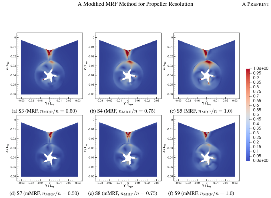
[§3.1 and §4.3] The Taylor–Couette verification in Sec. 3.1 cannot test the new term in Eq. (19), because u_MRF·∇f=0 there by axisymmetry, as the paper itself notes. The first nontrivial exercise of this term is the JBC self-propulsion case, but Sec. 4.3 selects q=0.8 and k=30 by comparing K_T and K_Q against the sliding-interface solution F01 (Table 5), and the same F01 solution is later used as the reference for the disc-averaged deviation metric in Eq. (35) and Table 8. The reported reductions R_ε≈0.58–0.83 are therefore in-sample measures: they compare a calibrated model against the calibration reference. To make the central local-accuracy claim load-bearing, the authors should either provide an independent test case in which ∇f is active and a known or experimentally measured solution exists, or demonstrate that the qualitative conclusions are insensitive to q and k over a wide range, or evaluate the local deviations against an independent reference (e.g., EFD fields) rather than only the SI solution.
[§2.2.1, Eq. (21)] With the selected parameters q=0.8 and k=30, Eq. (21) gives f≈(1+e^6)^-1≈2.5×10^-3 at d_int=0, not zero. Hence the compatibility condition (20) is satisfied only approximately at the interface, and the abstract's claim that mMRF "restores velocity and pressure continuity" is stronger than what is implemented. The residual discontinuity is small but nonzero, and its magnitude should be quantified in the manuscript. The authors should also discuss whether forcing f to exactly zero at the interface (e.g., by using a compactly supported damping function) would change the reported improvements.
[Eq. (19) and Appendix A] The derivation of the absolute-velocity formulation (19) is algebraically plausible, but it is presented in a condensed form that is difficult to audit. In particular, the step leading to Eq. (41) involves a rearrangement of the convective term that is not fully explained. Since the entire method rests on this equation, the authors should either expand the derivation in Appendix A to show each cancellation explicitly or provide a supplementary symbolic algebra check. This is not a request for cosmetic changes; it is needed to rule out a hidden sign or factor error in the extra ∇f term.

minor comments (6)

[Abstract and Sec. 2.2.1] The phrase "restoring velocity and pressure continuity" should be qualified as approximate, given that f does not vanish at the interface for the chosen sigmoid parameters (see major comment).
[Fig. 1 caption] The caption refers to the middle panel as "an unmodified simulation with a partially rotating grid"; for clarity it should state that this is classical MRF with n_MRF/n=0.5, consistent with the terminology used elsewhere in the paper.
[Sec. 4.3, Table 5] The table reports ΔK_T and ΔK_Q as percentages but uses the notation "0.944%" without a plus sign for positive values; using a consistent signed percentage format (e.g., +0.944%) would avoid ambiguity.
[Appendix B, Tables 9 and 10] The convergence ratios R=0.67 and R=0.40 for the grid and time-step studies are reported without a confidence interval; stating the number of significant digits and the definition of R exactly as in Eq. (44) is fine, but the authors should note that these are single-computation estimates and not based on a Richardson-extrapolation uncertainty calculation.
[Sec. 4.5 and Figs. 21–24] The EFD data in these figures are stated to be time-averaged experimental measurements, while the numerical fields are instantaneous at a common phase (for the deviation metric) or time-averaged over one revolution (for the contour comparisons). The caption should state clearly which averaging is used in each panel, since the mixing of instantaneous and averaged fields can mislead the reader.
[References] The reference to Durasević et al. (2022, 2023) is cited in the text as "Durasevi´c et al. (2022; 2023)" but appears in the reference list as "Durasevi´c, S., Gatin, I., Uroi´c, T., and Jasak, H."; please ensure consistent spelling and formatting.

Circularity Check

2 steps flagged · score 4.0 of 10

Local-accuracy claim is not independently supported: the Taylor-Couette verification cannot activate the new ∇f term, and the q,k parameters are calibrated to the same SI reference used for the local deviation metric.

fitted input called prediction [Sec. 4.3 (Table 5) and Sec. 4.5 (Eq. 35, Table 8)]
"Table 5 shows that, among the tested parameter combinations, the combination q=0.8 and k=30 (F10) exhibits the best agreement with the SI solution and is therefore selected for further use."

The free parameters q and k of the sigmoid scaling function f (Eq. 21) are selected by comparing integral KT/KQ values against the sliding-interface solution of the same JBC self-propulsion setup. The later local-accuracy headline is then measured as the disc-averaged deviation from that same SI solution (Eq. 35, Table 8). The reported error reductions (R_ε ≈ 0.58–0.83) are therefore in-sample: q,k were chosen to make the mMRF results agree with SI on integral quantities, and the local comparison uses the same reference solution. This is not a fully forced prediction because the fit target is integral while the evaluation is local, but the local improvement claim is not a blind, parameter-free test.
other [Sec. 3.1 (Taylor-Couette verification)]
"Due to the axial symmetry of the flow field (27), the compatibility relation (13) is maintained and uMRF·∇f=0. Therefore, the sliding interface (SI), moving reference frame (MRF), modified moving reference frame (mMRF) simulations should always produce identical velocity fields."

The only analytical verification explicitly renders the novel term (∇f·u_MRF)u inactive. The mMRF result is therefore identical to the classical MRF result by symmetry, and this exercise cannot validate the new physical contribution of the method. The first configuration in which the ∇f term actually acts is the JBC self-propulsion case, but there q and k are calibrated against the SI reference. Consequently, the central claim that mMRF reduces interface artifacts lacks an independent verification that isolates the new term from parameter calibration.

full rationale

The derivation of the modified governing equation is self-contained algebra from the stated spatially varying rotation-rate ansatz (Eqs. 14–19), so the method is not circular at the level of equation derivation. However, the paper's headline local improvement is not independently tested. The Taylor-Couette verification cannot exercise the new ∇f term, as the paper itself notes. In the JBC application, the sigmoid parameters q and k are chosen as the combination with the best agreement with the SI solution (F10 in Table 5), and the same SI solution is used as the reference for the disc-averaged local deviation (Eq. 35, Table 8). That makes the local-accuracy comparison partly a calibrated, in-sample evaluation rather than a prediction. The effect is tempered because the calibration target is integral (KT, KQ) and the advertised reduction is local, so the reduction is not forced by construction. In addition, Eq. (21) with q=0.8 and k=30 gives f≈(1+e^6)^-1≈2.5×10^-3 at d_int=0, so the implemented scaling function does not strictly vanish at the interface and Eq. (20) is only approximately satisfied; the abstract's 'restoring continuity' overstates the implemented boundary condition. Overall, the integral self-propulsion results are credible and externally anchored to EFD, but the central local artifact-reduction claim should be scored as partially circular: score 4.

Assumptions & free parameters 3 free parameters · 6 assumptions · 1 invented entities

The central method introduces two fitted parameters q,k and a modeling assumption that the nabla f source term is physically representative. Other assumptions are standard CFD or naval-architecture domain assumptions. No new physical entities or forces are postulated.

free parameters (3)

q = 0.8
Transition center position in the sigmoid scaling function f (Eq. 21); selected in Sec. 4.3 as the value giving closest agreement with the sliding-interface solution (F10) among q=0.4, 0.6, 0.8.
k = 30
Steepness of the sigmoid transition; selected in Sec. 4.3 together with q to minimize K_T and K_Q deviation from the SI reference (F10 among k=20, 30, 40).
PID gains K_P, K_I, K_D = 0.5e-2, 0.5e-5, 0.5e-4
Empirically tuned controller gains (Sec. 4.4) used to drive the self-propulsion rotation rate; they affect convergence behavior but not the final converged integral quantities directly.

assumptions (6)

domain assumption Incompressible RANS with Boussinesq eddy-viscosity closure (SST k-omega) is an adequate model for propeller-hull flow.
Secs. 2.1 and 2.3; all numerical results depend on this turbulence modeling assumption.
ad hoc to paper The propeller rotation can be decomposed into a grid-resolved part and an MRF part, with the MRF rate scaled by a position-only function f(r)=f_R(r_R).
Sec. 2.2 and Eq. (15); this is the central modeling construction and is not derived from blade mechanics.
ad hoc to paper The extra momentum term (nabla f dot u_MRF) u in Eq. (19) is the correct physical representation of a spatially varying frame rotation.
Assumed when writing Eq. (43); not tested independently because the Taylor-Couette case makes the term vanish.
domain assumption Compatibility at the interface is sufficient if f=0 there (Eq. 20).
Sec. 2.2; this ensures the frame source terms vanish at the boundary, but it does not guarantee zero artifacts inside the transition band.
domain assumption The thrust identity method, plus the experimental form factor and skin friction correction, gives valid propulsion factors.
Sec. 4.4; a standard naval architecture procedure used to derive 1-t, 1-w_T, and eta_R.
domain assumption Wave resistance from the bare-hull two-phase simulation can be added to the single-phase double-body self-propulsion simulation without propeller interaction.
Sec. 4.2 assumes the wave field is not significantly affected by the propeller.

invented entities (1)

Spatially varying reference-frame rotation scaling f(r)
purpose: Damps the MRF rotation from 1 near the propeller to 0 at the domain interface, replacing an abrupt MRF jump with a smooth transition.
The sigmoid form and parameters q,k are constructed for this method; no external data constrain f, and the verification case cannot isolate its effect because u_MRF dot nabla f = 0 there.

how reviews work

0 comments

Cite this review

Pith. "Pith review of A Modified Moving Reference Frame Method for Propeller Resolution." pith.science (2026). https://pith.science/paper/4XXV6U6J

@misc{pith2026260724630,
  author       = {Pith},
  title        = {Pith review of: A Modified Moving Reference Frame Method for Propeller Resolution},
  year         = {2026},
  howpublished = {\url{https://pith.science/paper/4XXV6U6J}},
  note         = {Machine review of arXiv:2607.24630}
}

abstract

Accurate resolution of propeller-hull interaction is essential for predicting the self-propulsion point in ship CFD, yet motion-resolving methods such as sliding interfaces (SI) are computationally expensive, while the classical Moving Reference Frame (MRF) approach cannot capture unsteady interaction effects. Partially rotating grid methods bridge this gap by splitting the propeller rotation into a grid-resolved and an MRF component, but the abrupt transition between the rotating and stationary domains introduces discontinuities in the velocity field. This work presents a modified MRF (mMRF) formulation in which the reference-frame rotation rate is scaled by a spatially varying function that decays smoothly from unity near the propeller to zero at the domain interface, restoring velocity and pressure continuity across the boundary. The governing equations are derived and implemented in the RANS solver FreSCo$^+$, verified against the analytical Taylor--Couette solution, and applied to open-water propeller and Japan Bulk Carrier self-propulsion simulations at model scale. Both MRF and mMRF reproduce the principal integral propulsion quantities ($n$, $K_{\mathrm{T}}$, $K_{\mathrm{Q}}$, $1-t$, $1-w_{\mathrm{T}}$, $\eta_{\mathrm{R}}$) accurately, but the mMRF markedly reduces interface discontinuities and non-physical artifacts in the local flow field, particularly at large MRF fractions, at essentially the same computational cost.

Figures

Figures reproduced from arXiv: 2607.24630 by the authors.

**Figure 2.** Computational setup for the Taylor–Couette flow verification case and evolution of the scaling function [PITH_FULL_IMAGE:figures/full_fig_p007_2.png] view at source ↗

**Figure 3.** Comparison of computed azimuthal velocities and pressure values with analytical results ( [PITH_FULL_IMAGE:figures/full_fig_p008_3.png] view at source ↗

Figures from the paper (21 more)

**Figure 4.** Figure 4: Illustration of the investigated JBC hull and propeller geometry. [PITH_FULL_IMAGE:figures/full_fig_p009_4.png]

**Figure 5.** Figure 5: Computational domain and boundary conditions for the open-water propeller simulation. The propeller is [PITH_FULL_IMAGE:figures/full_fig_p010_5.png]

**Figure 6.** Figure 6: Open water propeller curves for the non-dimensional thrust [PITH_FULL_IMAGE:figures/full_fig_p011_6.png]

**Figure 7.** Figure 7: Comparison of non-dimensional computational efforts associated with the MRF and the mMRF approaches [PITH_FULL_IMAGE:figures/full_fig_p012_7.png]

**Figure 8.** Figure 8: Computational domain and boundary conditions for the JBC bare-hull configurations, exploiting a [PITH_FULL_IMAGE:figures/full_fig_p013_8.png]

**Figure 9.** Figure 9: Computational grid for the two-phase flow resistance case. The mesh is refined in nested zones around the [PITH_FULL_IMAGE:figures/full_fig_p014_9.png]

**Figure 10.** Figure 10: Comparison of predicted and measured JBC bare hull towing test wave elevations. [PITH_FULL_IMAGE:figures/full_fig_p015_10.png]

**Figure 11.** Figure 11: Contour plots of the scaling function value at an exemplary cylindrical cross-section at [PITH_FULL_IMAGE:figures/full_fig_p016_11.png]

**Figure 12.** Figure 12: Blade thrust coefficients over propeller position for different mMRF parameters. [PITH_FULL_IMAGE:figures/full_fig_p017_12.png]

**Figure 13.** Figure 13: Computational domain and boundary conditions for the JBC self-propulsion simulation. The full breadth [PITH_FULL_IMAGE:figures/full_fig_p019_13.png]

**Figure 14.** Figure 14: Flowchart of the propeller rotation-rate control algorithm. [PITH_FULL_IMAGE:figures/full_fig_p020_14.png]

**Figure 15.** Figure 15: Example operation of the PID controller used to reach the self-propulsion point. The thrust–drag imbalance [PITH_FULL_IMAGE:figures/full_fig_p020_15.png]

**Figure 16.** Figure 16: Velocity-magnitude contour plots in the downstream ( [PITH_FULL_IMAGE:figures/full_fig_p022_16.png]

**Figure 17.** Figure 17: Contour plots of the normalized velocity-magnitude deviation from the SI solution (SP1), cf. Eqn. ( [PITH_FULL_IMAGE:figures/full_fig_p023_17.png]

**Figure 18.** Figure 18: Contour plots of the normalized velocity-magnitude deviation from the SI solution (SP1), cf. Eqn. ( [PITH_FULL_IMAGE:figures/full_fig_p024_18.png]

**Figure 19.** Figure 19: Contour plots of the normalized velocity-magnitude deviation from the SI solution (SP1), cf. Eqn. ( [PITH_FULL_IMAGE:figures/full_fig_p025_19.png]

**Figure 20.** Figure 20: Propeller grid cross-sections at r/RP = 0.344 at three refinement levels. The sensitivity study of the numerical results to the spatial and temporal discretization is performed for the OW1 open-water propeller case ( [PITH_FULL_IMAGE:figures/full_fig_p028_20.png]

**Figure 21.** Figure 21: Axial velocity contours in the downstream plane ( [PITH_FULL_IMAGE:figures/full_fig_p030_21.png]

**Figure 22.** Figure 22: Axial velocity contours in the upstream plane ( [PITH_FULL_IMAGE:figures/full_fig_p031_22.png]

**Figure 23.** Figure 23: Cross-plane velocity vectors in the downstream plane ( [PITH_FULL_IMAGE:figures/full_fig_p032_23.png]

**Figure 24.** Figure 24: Cross-plane velocity vectors in the upstream plane ( [PITH_FULL_IMAGE:figures/full_fig_p033_24.png]

Review history (2 revisions) →

Discussion (0). Continue with ORCID to comment.

Reference graph

Works this paper leans on

2 extracted references · 2 canonical work pages

[1]

Bakica, A., Gatin, I., Vuk ˇcevi´c, V ., Jasak, H., and Vladimir, N. (2019). Accurate assessment of ship-propulsion characteristics using CFD.Ocean Engineering, 175:149–162. Benek, J. A., Steger, J. L., and Dougherty, F. C. (1983). A flexible grid embedding technique with application to the Euler equations. InProceedings of the 6th AIAA Computational Flui...

work page 2019
[2]

1978 ITTC performance prediction method

International Towing Tank Conference (2021a). 1978 ITTC performance prediction method. ITTC Recommended Procedure 7.5-02-03-01.4. International Towing Tank Conference (2021b). Uncertainty analysis in CFD verification and validation, methodology and procedures. ITTC Recommended Procedure 7.5-03-01-01. Kawamura, T., Miyata, H., and Mashimo, K. (1997). Numer...

work page 2021

Pith tools

Reviewed August 15, 2026 · model on record in the stance chip above.

[1] [1]

Bakica, A., Gatin, I., Vuk ˇcevi´c, V ., Jasak, H., and Vladimir, N. (2019). Accurate assessment of ship-propulsion characteristics using CFD.Ocean Engineering, 175:149–162. Benek, J. A., Steger, J. L., and Dougherty, F. C. (1983). A flexible grid embedding technique with application to the Euler equations. InProceedings of the 6th AIAA Computational Flui...

work page 2019

[2] [2]

1978 ITTC performance prediction method

International Towing Tank Conference (2021a). 1978 ITTC performance prediction method. ITTC Recommended Procedure 7.5-02-03-01.4. International Towing Tank Conference (2021b). Uncertainty analysis in CFD verification and validation, methodology and procedures. ITTC Recommended Procedure 7.5-03-01-01. Kawamura, T., Miyata, H., and Mashimo, K. (1997). Numer...

work page 2021