REVIEW 4 major objections 5 minor 51 references
Biases in retrieving planetary signals in the presence of quasi-periodic stellar activity
T0 review · 4 major / 5 minor · reviewed 2026-08-14 · deepseek-v4-flash
Pith's one-line read When a low-mass planet's orbital period nears the star's rotation period, Gaussian-process activity correction can overestimate the planet's Doppler amplitude by 100% or more, with detection significance below 2 sigma even after two…
desk verdict A competent, useful simulation study quantifying GP-activity bias on small-planet RVs; the matched-kernel caveat is real but scoped, not fatal. read the letter →
The pith
A machine-rendered reading of the paper's core claim, the machinery that carries it, and where it could break.
The reading
What carries the argument
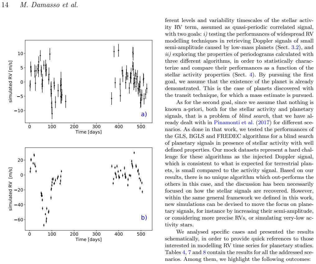
The load-bearing object is the quasi-periodic Gaussian process covariance kernel $$K(t,t') = $h^{2}$ \exp\left[-\frac{(t-t')^2}{2\tau_{\rm AR}^2} - \frac{\$sin^{2}$\left(\frac{\pi(t-t')}{P_{\rm rot}}\right)}{$2w^{2}$}\right] + \sigma_{\rm RV}^2(t)\delta_{t,t'},$$ where $h$ is the activity amplitude, $P_{\rm rot}$ the stellar rotation period, $w$ the periodic length scale, and $\tau_{\rm AR}$ the active-region evolutionary timescale. This kernel both generates the mock stellar activity, via random draws from the GP prior, and serves as the model used to fit it, so the experiment measures how well the recovery pipeline inverts the same stochastic process that created the data. Around that kernel the paper builds an injection-recovery Monte Carlo: 80,000 mock datasets in 16 scenarios, varying activity level, rotation period, activity timescale, period coincidence between planet and star, and one versus two observing seasons, analyzed with nested-sampling GP fits and three periodogram algorithms.
What would settle it
Re-run the Case III scenario (active star, $P_{\rm orb}\approx P_{\rm rot}$, $\tau_{\rm AR}\approx P_{\rm rot}$, two seasons) with the injected activity drawn from a physical rotating-spot or granulation model instead of sampled from the same GP kernel. If the median $K_b$ ratio then falls well below 2, the claimed 100% overestimate is partly an artifact of the matched kernel; if it stays near 2, the bias persists outside the paper's model-fidelity assumption.
Extended reading notes
Core claim
The paper's central claim is that when stellar activity is modeled as a quasi-periodic Gaussian process, the standard GP regression procedure used to remove it does not reliably retrieve a 1 m/s planetary signal. For the most difficult case, an active star whose rotation period nearly equals the planet's orbital period, the posterior median of the semi-amplitude runs about 1.9--2.1 times the injected value when the activity evolves on the rotation timescale, even with two seasons; with long-lived active regions the overestimate drops to about 20% but remains present. The detection significance is about 1.5--1.6 sigma across active-star cases, formally a non-detection. For quiet stars the median is generally close to the true value, and the 68.3rd percentile of the $K_b$ posterior often gives a more accurate estimate than the median. The paper frames these numbers as expected biases for transit-follow-up mass measurements and as a warning that better constraints on the activity model do not translate into better planetary amplitudes.
Load-bearing premise
The whole exercise assumes that a quasi-periodic Gaussian process kernel faithfully represents stellar activity, because the same kernel generates the mock signals and is then used to remove them; if real activity contains granulation, convection, or evolving spot geometries, the bias sizes could differ.
Editorial extensions
If this is right
- For active stars with $P_{\rm orb}\approx P_{\rm rot}$ and $\tau_{\rm AR}\approx P_{\rm rot}$, fitted $K_b$ values will be roughly twice the true amplitude even with two seasons of data, so mass estimates in these systems are systematically high.
- Across nearly all 16 scenarios, a 1 m/s planet is retrieved with significance below 2 sigma, meaning typical RV follow-up of small transiting planets will yield upper limits rather than detections.
- In quiet-star cases with $P_{\rm orb}$ well separated from $P_{\rm rot}$ and two seasons of data, the 68.3rd percentile of the $K_b$ posterior is closer to the injected value than the median is, so posterior upper limits are more trustworthy than best-fit medians.
- Adding a second season improves recovery of the activity timescale $\tau_{\rm AR}$ but does not cure the planet-amplitude bias; better activity modeling does not automatically produce better planet masses.
- Blind periodogram searches recover the planetary period in fewer than about 5 percent of datasets, so periodogram peaks alone cannot establish the presence or amplitude of such planets.
Reading between the lines
- Beyond the paper: because the activity model is given its best possible chance here, with the same kernel used for generation and fitting, real activity containing granulation, convection, or evolving spot geometries would likely make the planet-activity separation harder rather than easier, so the Case III overestimate may be a floor rather than a ceiling.
- Beyond the paper: the same simulation machinery could be used to test whether adding photometry or spectroscopic activity indicators as extra GP inputs reduces the $K_b$ inflation; the paper sets up exactly such a controlled comparison without running it.
- Beyond the paper: the strong $P_{\rm orb}\approx P_{\rm rot}$ bias implies that population-level mass-radius studies should flag or down-weight planets whose orbital period is close to the stellar rotation period, a survey-level consequence the paper does not draw.
Signed reviews
Editorial analysis
A structured set of objections, weighed in public.
Referee Report
Summary. This paper presents an extensive injection-recovery study of radial velocity (RV) time series containing a small planetary signal (K_b = 1 m/s) embedded in quasi-periodic stellar activity. The authors generate 80,000 mock datasets across 16 scenarios that vary activity amplitude (h = 3 and 15 m/s), rotation period, active-region lifetime (short vs. long tau_AR), the proximity of P_orb to P_rot, and one versus two observing seasons. They fit each dataset with a Keplerian plus a quasi-periodic Gaussian-process (GP) activity term using MultiNest and GEORGE, and quantify the recovered K_b, the significance K_b/sigma, the GP hyperparameters, and the fitted jitter. They also analyze a subset of datasets with GLS, BGLS, and FREDEC periodograms to measure completeness and reliability in recovering P_rot and P_orb. The main claims are that for K_b = 1 m/s the detection significance is generally below 2-sigma, that K_b is severely overestimated (by factors up to ~2) for active stars with P_orb ~ P_rot and short tau_AR, that the 68.3rd percentile of the K_b posterior is often closer to the injected value than the median, and that simple periodogram searches have very low completeness for the planet signal.
Significance. If the results hold, they provide a useful quantitative caution for the RV follow-up of small transiting planets, particularly in the context of TESS and PLATO targets. The study's strengths are its large simulation volume (5,000 datasets per scenario), the systematic coverage of activity regimes, the use of a realistic observing calendar, the explicit robustness checks in Appendix B and Sect. 3.2.2, and the comparison of three widely used periodogram tools. The paper also makes the simulated datasets available, which is a practical contribution. The main limitation is that the activity signal is both generated and fitted with the same quasi-periodic GP kernel, so the quoted bias magnitudes are matched-kernel estimates; the paper acknowledges this in Sect. 2.2 and Sect. 3.1, but the practical conclusions in Sect. 5 are stated more broadly. Subject to that caveat, the internal statistics are solid and the reported trends are clearly tabulated.
major comments (4)
- [Sect. 3.2, Case III and Table 4] The headline statement in Case III, 'The semi-amplitude Kb is overestimated by 100% or more when tau_AR is close to P_rot, even with two seasons of data,' is not fully supported by Table 4. In the active-star, P_orb~P_rot, short-tau_AR row, K_b,ratio,50% is 2.14+0.5-0.4 for one season, but 1.9+0.5-0.4 for two seasons, so the median two-season overestimate is about 90%, not 100% or more. Please rephrase the claim to state the median overestimate (or identify the percentile that exceeds 100%).
- [Sect. 2.5 and Sect. 3.1] The activity term is generated by drawing from the same quasi-periodic GP kernel (Eq. 1) used in the retrieval, so Table 4 measures bias under a matched-kernel, model-true protocol. The manuscript acknowledges in Sect. 2.2 that the quasi-periodic representation is 'not necessarily complete' and in Sect. 3.1 that the kernel choice is a working hypothesis, but the abstract and Sect. 5 draw practical conclusions about real surveys. Real activity includes granulation, convection, differential rotation, and complex spot evolution, all of which could change the bias magnitudes and the conclusions about GP effectiveness. I recommend either adding robustness simulations with a different activity generator (e.g., a spot-occultation model or a GP with a different kernel) or explicitly restricting the central claims to the exactly quasi-periodic case.
- [Sect. 3.2, 'Upper limits as defined by the 68th percentile'] Describing the 68.3rd percentile of the K_b posterior as a 'more accurate estimate' is problematic in the low-signal cases treated here, where the posterior is one-sided and this percentile is an upper limit rather than a point estimate. The comparison in Table 4 does not establish accuracy; a coverage statistic, such as the fraction of datasets for which the 68.3% credible interval contains the injected K_b, would be a more meaningful calibration. This issue affects one of the summary bullets in Sect. 5.
- [Table 3 and Sect. 3.2] The quantity K_b,50%/sigma_Kb^- is repeatedly called a 'detection significance,' but for one-sided posteriors that pile up near zero, the lower uncertainty sigma_Kb^- can be very small, making this ratio a poor proxy for significance relative to a null amplitude. The statement that detection significance 'stays below 2 sigma' should be justified or the quantity should be renamed, for example 'median-over-lower-uncertainty ratio.'
minor comments (5)
- [Sect. 4] The text '1 0000 RV mock datasets' should read '10 000 RV mock datasets.'
- [Table 5] The line 'median sigma_jit, no GP/sigma_jit, with GP' is duplicated within each observing-season block; remove the repeated rows.
- [Table 8] In the low-activity, short-tau_AR, two-season GLS row, the entry '30.9.4%' should be '30.9%.'
- [Section 1] There is a typo in the introduction: 'Zeng et al. 017b' should be 'Zeng et al. 2017b.'
- [Sections 2.1 and 2.5] The notation alternates between K_p (Sect. 2.1) and K_b (Sect. 2.5 onward) for the planetary semi-amplitude; please use a single symbol throughout.
Circularity Check
No significant circularity: the matched-kernel protocol is an explicitly stated modeling assumption, and the bias results are conditional claims, not self-fulfilling by construction.
full rationale
The paper is an injection-recovery simulation study, and it repeatedly and explicitly conditions its conclusions on the quasi-periodic GP kernel. Mock activity is drawn from Eq. (1) using the GEORGE sample function, and the retrieval fits the same kernel, with the stated working hypothesis that this kernel choice is justified (Sect. 3.1). This is a model-fidelity assumption rather than a circular derivation: the bias statistics for Kb, tau_AR, sigma_jit, and the periodogram completeness/reliability figures are computed from the simulated data and are not imposed by the definitions of the injected parameters. The paper is also transparent that the quasi-periodic model is 'only one of several possible representations of the stellar component in RV time series' and that it lacks the detail of Dumusque (2016), including granulation and oscillations. The self-citations (Pinamonti et al. 2017, Damasso & Del Sordo 2017, Pinamonti et al. 2018) are used for conventions, prior choices, and algorithm comparisons, but the central bias map does not rest on accepting an unverified self-cited theorem. No step in the derivation chain reduces by construction to its own inputs, so the honest finding is no significant circularity.
Assumptions & free parameters
free parameters (8)
- Planet semi-amplitude Kb =
1 m/s fixed; 2 and 3 m/s in exploratory subsets
- Stellar activity amplitude h =
3 m/s (low activity), 15 m/s (high activity)
- RV uncertainty sigma_RV =
N(2, 0.3^2) m/s
- Stellar rotation period P_rot =
20 d (low activity), 10 d (active)
- Active region timescale tau_AR =
P_rot (short) and 10*P_rot (long)
- Number of epochs per season =
40 (one season) or 80 (two seasons)
- P_orb prior width in MC fit =
P_sim +/- 0.5 d
- tau_AR prior in MC fit =
U(0,1000) d linear; log-uniform variant explored
assumptions (5)
- domain assumption The quasi-periodic GP kernel (Eq. 1) is a realistic representation of stellar activity in RV time series.
- domain assumption Planets in the simulation are on circular orbits.
- domain assumption Data are collected with a single instrument and noise is Gaussian with known sigma_RV, plus an optional fitted jitter.
- standard math Bayesian sampling with MultiNest over the parameter space yields correct posterior estimates.
- domain assumption The orbital period is known from transits to within 0.5 days and P_rot to within 5 days for the MC analysis.
Cite this review
Pith. "Pith review of Biases in retrieving planetary signals in the presence of quasi-periodic stellar activity." pith.science (2026). https://pith.science/paper/4ZWOTNGD
@misc{pith2026190802217,
  author       = {Pith},
  title        = {Pith review of: Biases in retrieving planetary signals in the presence of quasi-periodic stellar activity},
  year         = {2026},
  howpublished = {\url{https://pith.science/paper/4ZWOTNGD}},
  note         = {Machine review of arXiv:1908.02217}
}
abstract
Gaussian process regression is a widespread tool used to mitigate stellar correlated noise in radial velocity time series. It is particularly useful to search for and determine the properties of signals induced by small-size, low-mass planets ($R_p<4R_{\rm \oplus}$, $m_p<10M_{\rm \oplus}$). By using extensive simulations based on a quasi-periodic representation of the stellar activity component, we investigate the ability in retrieving the planetary parameters in 16 different realistic scenarios. We analyse systems composed by one planet and host stars having different levels of activity, focusing on the challenging case represented by low-mass planets, with Doppler semi-amplitudes in the range 1-3 $m s^{-1}$. We consider many different configurations for the quasi-periodic stellar activity component, as well as different combinations of the observing epochs. We use commonly-employed analysis tools to search for and characterize the planetary signals in the datasets. The goal of our injection-recovery statistical analysis is twofold. First, we focus on the problem of planet mass determination. Then, we analyse in a statistical way periodograms obtained with three different algorithms, in order to explore some of their general properties, as the completeness and reliability in retrieving the injected planetary and stellar activity signals with low false alarm probabilities. This work is intended to provide some understanding of the biases introduced in the planet parameters inferred from the analysis of radial velocity time series that contain correlated signals due to stellar activity. It also aims to motivate the use and encourage the improvement of extensive simulations for planning spectroscopic follow-up observations.
Figures


Figures from the paper (5 more)


Reference graph
Works this paper leans on
-
[1]
Affer L., et al., 2016, @doi [ ] 10.1051/0004-6361/201628690 , http://adsabs.harvard.edu/abs/2016A
-
[2]
Agol E., Fabrycky D. C., 2017, Transit-Timing and Duration Variations for the Discovery and Characterization of Exoplanets . p. 7, @doi 10.1007/978-3-319-30648-3_7-1
-
[3]
Ambikasaran S., Foreman-Mackey D., Greengard L., Hogg D. W., O'Neil M., 2014
work page 2014
-
[4]
Artigau \'E ., et al., 2014, in Ground-based and Airborne Instrumentation for Astronomy V. p. 914715 ( @eprint arXiv 1406.6992 ), @doi 10.1117/12.2055663
arXiv 2014
-
[5]
Baluev R. V., 2013, @doi [Astronomy and Computing] 10.1016/j.ascom.2013.11.003 , http://adsabs.harvard.edu/abs/2013A
-
[6]
Barclay T., Pepper J., Quintana E. V., 2018, @doi [ ] 10.3847/1538-4365/aae3e9 , https://ui.adsabs.harvard.edu/abs/2018ApJS..239....2B 239, 2
-
[7]
Online at <A href=``href=''>https://pos.sissa.it/cgi-bin/reader/conf.cgi?confid=269</A>, id.69
Benatti S., et al., 2016, in Frontier Research in Astrophysics II, held 23-28 May, 2016 in Mondello (Palermo), Italy (FRAPWS2016). Online at <A href=``href=''>https://pos.sissa.it/cgi-bin/reader/conf.cgi?confid=269</A>, id.69. p. 69
work page 2016
-
[8]
A., Huber D., Gaidos E., van Saders J
Berger T. A., Huber D., Gaidos E., van Saders J. L., 2018, @doi [ ] 10.3847/1538-4357/aada83 , https://ui.adsabs.harvard.edu/abs/2018ApJ...866...99B 866, 99
Show all 51 references
-
[9]
Buchner J., et al., 2014, @doi [ ] 10.1051/0004-6361/201322971 , http://adsabs.harvard.edu/abs/2014A
2014 doi
-
[10]
Damasso M., Del Sordo F., 2017, @doi [ ] 10.1051/0004-6361/201630050 , http://adsabs.harvard.edu/abs/2017A
2017 doi
-
[11]
Damasso M., et al., 2018, @doi [ ] 10.1051/0004-6361/201732459 , 615, A69
2018 doi
-
[12]
Damasso M., et al., 2019, @doi [ ] 10.1051/0004-6361/201834671 , 624, A38
2019 doi
-
[13]
Dumusque X., 2016, @doi [ ] 10.1051/0004-6361/201628672 , http://adsabs.harvard.edu/abs/2016A
2016 doi
-
[14]
Dumusque X., et al., 2017, @doi [ ] 10.1051/0004-6361/201628671 , http://adsabs.harvard.edu/abs/2017A
2017 doi
-
[15]
Feng F., Tuomi M., Jones H. R. A., Butler R. P., Vogt S., 2016, @doi [ ] 10.1093/mnras/stw1478 , http://adsabs.harvard.edu/abs/2016MNRAS.461.2440F 461, 2440
2016 doi
-
[16]
T., Hobson M
Feroz F., Balan S. T., Hobson M. P., 2011, @doi [ ] 10.1111/j.1365-2966.2011.18962.x , https://ui.adsabs.harvard.edu/abs/2011MNRAS.415.3462F 415, 3462
2011
-
[17]
P., Cameron E., Pettitt A
Feroz F., Hobson M. P., Cameron E., Pettitt A. N., 2013, preprint, http://adsabs.harvard.edu/abs/2013arXiv1306.2144F ( @eprint arXiv 1306.2144 )
2013 arXiv
-
[18]
A., et al., 2016, @doi [ ] 10.1088/1538-3873/128/964/066001 , http://adsabs.harvard.edu/abs/2016PASP..128f6001F 128, 066001
Fischer D. A., et al., 2016, @doi [ ] 10.1088/1538-3873/128/964/066001 , http://adsabs.harvard.edu/abs/2016PASP..128f6001F 128, 066001
2016 doi
-
[19]
J., Petigura E
Fulton B. J., Petigura E. A., 2018, @doi [ ] 10.3847/1538-3881/aae828 , https://ui.adsabs.harvard.edu/abs/2018AJ....156..264F 156, 264
2018 doi
-
[20]
J., et al., 2017, @doi [ ] 10.3847/1538-3881/aa80eb , http://adsabs.harvard.edu/abs/2017AJ....154..109F 154, 109
Fulton B. J., et al., 2017, @doi [ ] 10.3847/1538-3881/aa80eb , http://adsabs.harvard.edu/abs/2017AJ....154..109F 154, 109
2017 doi
-
[21]
D., et al., 2018, @doi [ ] 10.3847/1538-3881/aab8f3 , http://adsabs.harvard.edu/abs/2018AJ....155..203H 155, 203
Haywood R. D., et al., 2018, @doi [ ] 10.3847/1538-3881/aab8f3 , http://adsabs.harvard.edu/abs/2018AJ....155..203H 155, 203
2018 doi
-
[22]
Jurgenson C., Fischer D., McCracken T., Sawyer D., Szymkowiak A., Davis A., Muller G., Santoro F., 2016, in Ground-based and Airborne Instrumentation for Astronomy VI. p. 99086T ( @eprint arXiv 1606.04413 ), @doi 10.1117/12.2233002
2016 arXiv
-
[23]
D., Fortney J
Lopez E. D., Fortney J. J., 2014, The Astrophysical Journal, 792, 1
2014
-
[24]
Mahadevan S., et al., 2014, in Ground-based and Airborne Instrumentation for Astronomy V. p. 91471G, @doi 10.1117/12.2056417
2014 doi
-
[25]
Malavolta L., et al., 2018, @doi [ ] 10.3847/1538-3881/aaa5b5 , http://adsabs.harvard.edu/abs/2018AJ....155..107M 155, 107
2018 doi
-
[26]
Marconi A., et al., 2016, in Ground-based and Airborne Instrumentation for Astronomy VI. p. 990823 ( @eprint arXiv 1609.00497 ), @doi 10.1117/12.2231653
2016 arXiv
-
[27]
S., et al., 2018, @doi [ ] 10.1051/0004-6361/201732143 , http://adsabs.harvard.edu/abs/2018A
Mascare \ n o A. S., et al., 2018, @doi [ ] 10.1051/0004-6361/201732143 , http://adsabs.harvard.edu/abs/2018A
2018 doi
-
[28]
P., Correia C
Mortier A., Faria J. P., Correia C. M., Santerne A., Santos N. C., 2015, @doi [ ] 10.1051/0004-6361/201424908 , http://adsabs.harvard.edu/abs/2015A
2015 doi
-
[29]
E., Ford E
Nelson B. E., Ford E. B., Buchner J., Cloutier R., D \' az R. F., Faria J. P., Rajpaul V. M., Rukdee S., 2018, preprint, http://adsabs.harvard.edu/abs/2018arXiv180604683N ( @eprint arXiv 1806.04683 )
2018 arXiv
-
[30]
E., 2019, @doi [Annual Review of Earth and Planetary Sciences] 10.1146/annurev-earth-053018-060246 , https://ui.adsabs.harvard.edu/abs/2019AREPS..47...67O 47, 67
Owen J. E., 2019, @doi [Annual Review of Earth and Planetary Sciences] 10.1146/annurev-earth-053018-060246 , https://ui.adsabs.harvard.edu/abs/2019AREPS..47...67O 47, 67
2019 doi
-
[31]
E., Wu Y., 2013, @doi [ ] 10.1088/0004-637X/775/2/105 , http://adsabs.harvard.edu/abs/2013ApJ...775..105O 775, 105
Owen J. E., Wu Y., 2013, @doi [ ] 10.1088/0004-637X/775/2/105 , http://adsabs.harvard.edu/abs/2013ApJ...775..105O 775, 105
2013 doi
-
[32]
Pepe F., et al., 2014, @doi [Astronomische Nachrichten] 10.1002/asna.201312004 , 335, 8
2014 doi
-
[33]
Perger M., et al., 2017, @doi [ ] 10.1051/0004-6361/201731307 , http://adsabs.harvard.edu/abs/2017A
2017 doi
-
[34]
S., Damasso M., 2017, @doi [ ] 10.1093/mnras/stx664 , http://adsabs.harvard.edu/abs/2017MNRAS.468.3775P 468, 3775
Pinamonti M., Sozzetti A., Bonomo A. S., Damasso M., 2017, @doi [ ] 10.1093/mnras/stx664 , http://adsabs.harvard.edu/abs/2017MNRAS.468.3775P 468, 3775
2017 doi
-
[35]
Pinamonti M., et al., 2018, @doi [ ] 10.1051/0004-6361/201732535 , http://adsabs.harvard.edu/abs/2018A
2018 doi
-
[36]
Quirrenbach A., et al., 2016, in Ground-based and Airborne Instrumentation for Astronomy VI. p. 990812, @doi 10.1117/12.2231880
2016 doi
-
[37]
Rauer H., et al., 2014, @doi [Experimental Astronomy] 10.1007/s10686-014-9383-4 , http://adsabs.harvard.edu/abs/2014ExA....38..249R 38, 249
2014 doi
-
[38]
C., Mayor M., Naef D., Pepe F., Queloz D., Udry S., Blecha A., 2000, , http://adsabs.harvard.edu/abs/2000A
Santos N. C., Mayor M., Naef D., Pepe F., Queloz D., Udry S., Blecha A., 2000, , http://adsabs.harvard.edu/abs/2000A
2000
-
[39]
Schwab C., et al., 2016, in Ground-based and Airborne Instrumentation for Astronomy VI. p. 99087H, @doi 10.1117/12.2234411
2016 doi
-
[40]
P., 2016, @doi [ ] 10.1093/mnras/stw1936 , http://adsabs.harvard.edu/abs/2016MNRAS.463.1844S 463, 1844
Stelzer B., Damasso M., Scholz A., Matt S. P., 2016, @doi [ ] 10.1093/mnras/stw1936 , http://adsabs.harvard.edu/abs/2016MNRAS.463.1844S 463, 1844
2016 doi
-
[41]
I., Esposito M., 2017, @doi [ ] 10.1093/mnras/stx771 , http://adsabs.harvard.edu/abs/2017MNRAS.468.4772S 468, 4772
Su \'a rez Mascare \ n o A., Rebolo R., Gonz \'a lez Hern \'a ndez J. I., Esposito M., 2017, @doi [ ] 10.1093/mnras/stx771 , http://adsabs.harvard.edu/abs/2017MNRAS.468.4772S 468, 4772
2017 doi
-
[42]
Van Eylen V., et al., 2019, @doi [ ] 10.3847/1538-3881/aaf22f , https://ui.adsabs.harvard.edu/abs/2019AJ....157...61V 157, 61
2019 doi
-
[43]
A., Ciardi D
Vanderburg A., Plavchan P., Johnson J. A., Ciardi D. R., Swift J., Kane S. R., 2016, @doi [ ] 10.1093/mnras/stw863 , http://adsabs.harvard.edu/abs/2016MNRAS.459.3565V 459, 3565
2016 doi
-
[44]
M., Marcy G
Weiss L. M., Marcy G. W., 2014, @doi [ ] 10.1088/2041-8205/783/1/L6 , http://adsabs.harvard.edu/abs/2014ApJ...783L...6W 783, L6
2014 doi
-
[45]
Wildi F., et al., 2017, in Society of Photo-Optical Instrumentation Engineers (SPIE) Conference Series. p. 1040018, @doi 10.1117/12.2275660
2017 doi
-
[46]
Wu Y., 2019, @doi [ ] 10.3847/1538-4357/ab06f8 , https://ui.adsabs.harvard.edu/abs/2019ApJ...874...91W 874, 91
2019 doi
-
[47]
Zechmeister M., K \"u rster M., 2009, @doi [ ] 10.1051/0004-6361:200811296 , http://adsabs.harvard.edu/abs/2009A
2009 doi
-
[48]
Zeng L., et al., 2017, in Lunar and Planetary Science Conference. p. 1576
2017
-
[49]
Zeng L., et al., 2019, arXiv e-prints, https://ui.adsabs.harvard.edu/abs/2019arXiv190604253Z
2019
-
[50]
B., Sasselov D
Zeng L., Jacobsen S. B., Sasselov D. D., 2017b, Research Notes of the AAS, 1, 32
-
[51]
write newline
" write newline "" before.all 'output.state := FUNCTION fin.entry write newline FUNCTION new.block output.state before.all = 'skip after.block 'output.state := if FUNCTION new.sentence output.state after.block = 'skip output.state before.all = 'skip after.sentence 'output.stat...
Reviewed August 14, 2026 · model on record in the stance chip above.
Discussion (0). Continue with ORCID to comment.