REVIEW 2 major objections 3 minor 96 references
A Two-Gauge Field Model for Magnetoelectric Boundaries
T0 review · 2 major / 3 minor · reviewed 2026-08-05 · deepseek-v4-flash
Pith's one-line read A coupled Maxwell and planar Chern-Simons field reproduces a magnetoelectric material boundary with two tunable parameters, and the exact propagator shows that in the strong-coupling limit the plane becomes a perfect conductor.
desk verdict A promising two-gauge-field construction, but the printed exact propagator has a block determinant in the numerator where it belongs in the denominator, so the central perfect-conductor limit does not follow as written. read the letter →
The pith
A machine-rendered reading of the paper's core claim, the machinery that carries it, and where it could break.
The reading
What carries the argument
The load-bearing object is a 2×2 matrix of differential operators built from the Maxwell block and the planar Maxwell-Chern-Simons block, joined by antisymmetric Chern-Simons mixing terms localized by δ(x3−a). The exact propagator is obtained by inverting this matrix through reduced propagators, i.e. propagators Fourier-transformed only in the directions parallel to the plane. The inversion hinges on the matrix M in Eq. (28), whose inverse enters every interaction computed later. A secondary mechanism is the reading of the delta-localized coupling as a surface polarization and magnetization induced by the planar field, which makes the magnetoelectric character of the model visible.
What would settle it
Compute the determinant or residue of the matrix M in Eq. (28) in a neighborhood of p∥²=m² and p∥=0 under the standard iε prescription: an unregulated pole would show up as a divergence in one of the integral representations of the interaction energies, such as Eq. (44) or Eq. (58), that the closed-form results do not contain. Alternatively, check Eq. (39) directly against the standard perfect-conductor boundary conditions, tangential E = 0 and normal B = 0 on the plane.
Extended reading notes
Core claim
On the paper's own terms, the central result is Eq. (38): the exact matrix propagator of the two-gauge-field system. The propagator is obtained by writing the action as a quadratic form with a 2×2 matrix of differential operators and solving the Green-function equation through reduced propagators in the coordinates parallel to the plane. All interaction corrections are packaged through a function χ(p∥) defined in Eq. (37). Taking μ→∞, the off-diagonal sectors decouple: the electromagnetic block becomes the free Maxwell propagator in Feynman gauge corrected by a perfectly conducting plane at x3=a, while the planar block becomes pure gauge and loses physical observables. The paper then reads c
Load-bearing premise
The derivation assumes the matrix M in Eq. (28) is invertible for every parallel momentum, in particular at p∥²=m² and p∥=0, with the Feynman iε prescription silently handling the poles; if that inverse develops extra unregulated poles, the exact propagator and all derived energies would be ill-defined.
Editorial extensions
If this is right
- In the strong-coupling limit the model's predictions reduce, by construction of the propagator, to image-charge electrostatics: a point charge is attracted to the plane with force −Q²/(16πR⊥²), independent of the Chern-Simons mass m.
- For finite μ and m the charge–plane force contains a term decaying more slowly than Coulomb plus a short-range term, so the boundary acts as a tunable attractive layer whose range shrinks as μ or m grows.
- Planar Chern-Simons charges interact like electromagnetism with a Yukawa-like kernel when μ=0; increasing μ suppresses planar propagation until, at μ→∞, all planar observables vanish.
- A stationary electric charge generates a magnetic field in the bulk and electric and magnetic fields in the plane, a concrete magnetoelectric signature that disappears when the Chern-Simons mass m goes to zero.
- Topological planar sources behave as Dirac points (time-like) or electric dipoles (space-like), and their anisotropic interaction produces a torque on the sources.
Reading between the lines
- Because μ continuously interpolates between a decoupled plane (μ=0) and a perfect conductor (μ→∞) while m tunes the magnetoelectric response, the model could be used to extract an effective surface conductivity or an axion-like θ for a boundary from the two parameters—a step the paper does not explicitly take.
- The exact propagator opens a direct route to Casimir-energy calculations for one or two such layers by summing zero-point fluctuations; in the strong-coupling limit that calculation should reproduce the standard perfect-conductor Casimir result, providing a clean cross-check.
- The same inversion technique should carry over to multiple parallel planes or to a smooth profile instead of a delta-layer: the matrix would grow, but the structure of the reduced-propagator equations would be unchanged.
- The field solutions suggest a direct experimental test: measure the magnetic field induced by a static charge near a candidate magnetoelectric material and compare its m-dependent amplitude to Eq. (74).
Editorial analysis
A structured set of objections, weighed in public.
Referee Report
Summary. The paper proposes a field-theoretic model of a magnetoelectric boundary: a 3+1-dimensional Maxwell field coupled through Chern-Simons-like terms, localized on a plane x3=a, to a planar Maxwell-Chern-Simons field. The central result is an exact propagator, Eq. (38), obtained by inverting a 2×2 block matrix of differential operators in Eq. (28). The authors claim that in the strong-coupling limit μ→∞ the electromagnetic sector reduces to the Maxwell propagator with a perfectly conducting plate, Eq. (39), while the planar sector becomes pure gauge, Eq. (40). The propagator is then used to compute charge-plane interactions, planar source-source interactions, topological-source interactions, and field solutions for a stationary charge. Several decoupling and massless limits are compared with known results.
Significance. The two-parameter structure of the model is conceptually appealing, and the paper provides explicit formulas for a wide class of observables. The μ=0 limit correctly reduces to the decoupled Maxwell plus planar Maxwell-Chern-Simons theory, and several m→∞ limits are consistent with the expected suppression of planar propagation. However, the central algebraic step—the inversion of M in Eq. (28)—is not demonstrated and, as printed, the resulting propagator is not the inverse of M. The claimed perfect-conductor limit therefore does not follow, and all subsequent interaction energies and field solutions inherit the issue. The paper ships no machine-checkable proof or numerical code, so the correctness of this algebra is essential and must be established explicitly.
major comments (2)
- [Section II, Eqs. (33)–(36) and (39)] The factor {1+p∥²[2χ(p∥)+χ(p∥)²(p∥²−m²)]} appears in the numerator of every element of ∆G. For the block matrix M=[[1,A],[B,1]] in Eq. (28), Schur-complement inversion gives (M^{-1})_{11}=(1−AB)^{-1}, etc. On the transverse subspace det(1−AB)=1+p∥²[2χ+χ²(p∥²−m²)], so this determinant must appear in the denominator, not the numerator. As printed, ∆G(11) at fixed p∥ is O(χ⁴)=O(μ⁸) as μ→∞, so Eq. (33) does not approach the image propagator and Eq. (39) is not a consequence. Equations (34)–(36) have the same structural error, so the claimed limits (39), (40) and every downstream result using this propagator—Eqs. (44), (45), (54), (58), (62), and (73)–(76)—are unsupported as written. If the determinant was intended in the denominator, the displayed expressions are misprinted; if it was intended in the numerator, they are not the inverse of Eq. (28). Either way, the central derivation needs to
- [Section II, Eqs. (27)–(32)] The inversion of M is not shown; the text says only 'performing some algebraic manipulations.' This is not a presentation quibble: the placement of the determinant is exactly the error identified above. Moreover, the pole structure is not discussed. The matrix M contains 1/(p∥²−m²) and 1/√(−p∥²), and the determinant itself develops a pole at p∥²=m² through χ. Since Secs. III–V integrate the propagator over momenta, the iε prescription and the domain of M^{-1} must be specified. Without this, the 'exact' character of Eq. (38) cannot be verified even after the algebraic sign issue is fixed.
minor comments (3)
- [Eq. (2) and Conclusions] The dimensional analysis in Eq. (2) gives [μ]=[ℓ]^{-1/2}, which is consistent with the use of μ² in χ. The Conclusions, however, state that μ has 'dimensions of mass squared.' Please correct the latter.
- [Throughout] There are several typos and leftover placeholders: 'collunm' before Eq. (14), 'refrence' in Sec. IV.C, and the word 'AQUI' appearing after Figs. 5 and 9. These should be cleaned up.
- [Sec. IV.A, after Eq. (54)] The text says 'opposite-sign sources q1q2 > 0 experience an attractive one'; the condition for attraction should be q1q2 < 0.
Circularity Check
No significant circularity: the propagator is obtained by inverting the model's kinetic operator, and later limits are consistency checks rather than fitted or assumed inputs.
full rationale
The paper's derivation chain starts from the Lagrangian (1) with free parameters m and mu; the propagator is defined as the inverse of the quadratic operator O in Eq. (17). Equations (26)-(30) are a standard reduced-propagator solution for the delta-localized interaction, and the displayed inverse (33)-(36) is the algebraic output of that inversion. None of the later results -- charge-plane energy (45), source-source energies (54), (58), (62), or field solutions (73)-(76) -- is used to fit m or mu; they are computed as integrals of the derived propagator with prescribed sources. The mu->infinity and mu=0 limits are consistency checks against the known perfect-conductor propagator [64] and Maxwell-Chern-Simons results [30]. Even where those references share authors with the present paper, they are external, previously established benchmarks rather than inputs to the derivation, and the present propagator is derived independently of those target limits. No parameter is fitted to the quantities being predicted, and no uniqueness theorem from prior same-author work is invoked to exclude alternatives. The 'AQUI' placeholders after Fig. 5 and Fig. 9 are editorial artifacts and do not alter this assessment. Whether the block-matrix inverse (33)-(36) is algebraically correct as printed -- e.g., whether the chi-bracket belongs in the numerator or denominator -- is a correctness and invertibility concern, not a circularity concern; an erroneous inverse would leave the strong-coupling claim unsupported, but that is the opposite of circularity.
Assumptions & free parameters
free parameters (2)
- m (Chern-Simons mass)
- mu (interfield coupling constant)
assumptions (5)
- domain assumption The planar Chern-Simons field A_bar obeys Maxwell-Chern-Simons dynamics with mass m.
- domain assumption A Dirac delta function localizes the planar field and its couplings to the plane x3 = a.
- standard math Feynman gauge (alpha = beta = 1) is a legitimate gauge choice for both fields.
- standard math The standard Feynman i-epsilon prescription regularizes propagator poles.
- ad hoc to paper The specific form of the Chern-Simons-like coupling with parameter mu is the correct minimal emulation of magnetoelectric boundaries.
invented entities (1)
-
Planar Chern-Simons gauge field A_bar_mu
Cite this review
Pith. "Pith review of A Two-Gauge Field Model for Magnetoelectric Boundaries." pith.science (2026). https://pith.science/paper/55TKTSBN
@misc{pith2026250821697,
  author       = {Pith},
  title        = {Pith review of: A Two-Gauge Field Model for Magnetoelectric Boundaries},
  year         = {2026},
  howpublished = {\url{https://pith.science/paper/55TKTSBN}},
  note         = {Machine review of arXiv:2508.21697}
}
read the original abstract
This work introduces a field-theoretical model designed to simulate the presence of material layers with magnetoelectric properties. The model comprises the standard Maxwell field coupled to a Chern-Simons field confined to a planar layer. The electromagnetic behavior of the boundary is emulated through the interaction between the Chern-Simons and Maxwell fields, governed by two parameters: the Chern-Simons mass and the coupling constant between the fields. Both parameters can be adjusted to reflect the specific properties of different materials. We compute the exact propagator of the theory and employ it to investigate several physical properties. Our analysis focuses on phenomena that arise from the presence of external sources coupled to both the Maxwell and Chern-Simons fields, considering various scenarios. In the Chern-Simons sector, the sources emulate defects in the crystal lattice of the material layer. The main objective of this paper is to present the proposed model and to explore its behavior in the simple context of a single planar material interface. We also suggest possible extensions of the model to more general configurations.
Figures


Figures from the paper (10 more)




Reference graph
Works this paper leans on
-
[1]
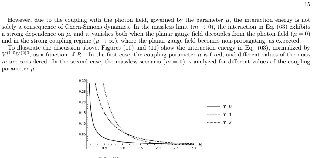
(63) We now present some remarks regarding the result above
Time-like case For the time-like case, the interaction energy (62) becomes EV (1)V (2) (m, µ, R∥) = V (1)0V (2)0 4 Re n 2 R∥ (µ2/8 + im)H−1((µ2/8 + im)R∥) + (µ2/8 + im)2 h Y0((µ2/8 + im)R∥) + H−2((µ2/8 + im)R∥) io . (63) We now present some remarks regarding the result above. In the temporal case, the topological source given by (61) is equivalent to a Di...
-
[2]
ˆR∥ V(2)
Space-like case In the spatial case, where V (1)0 = V (2)0 = 0, the interaction energy given by (62) becomes EV (1)V (2) (m, µ, R∥) = V(1).V(2) 4R∥ Re n (µ2/8 + im) h 2 H−1((µ2/8 + im)R∥) + 2Y1((µ2/8 + im)R∥) − (µ2/8 + im)R∥ H−2((µ2/8 + im)R∥) + Y0((µ2/8 + im)R∥) io + V(1). ˆR∥ V(2). ˆR∥ Re n (µ2/8 + im)2 × h H−2((µ2/8 + im)R∥) − Y2((µ2/8 + im)R∥) io , (6...
2024
-
[3]
Zhang, Int
S. Zhang, Int. J. Mod. Phys. B 06, 25 (1992)
1992
-
[4]
Banerjee, P
R. Banerjee, P. Mukherjee, Nucl. Phys. B 478, 235 (1996)
1996
-
[5]
Banerjee, P
R. Banerjee, P. Mukherjee, Prog. Theor. Phys. 101, 1189 (1999)
1999
-
[6]
Frohlich and A
J. Frohlich and A. Zee, Nucl. Phys. B 364, 517 (1991)
1991
-
[7]
de Gracia and B.M
G.B. de Gracia and B.M. Pimentel, Rev. Bras. Ens. Fis. 45, e20230042 (2023). 20
2023
-
[8]
Hasan and C.L
M.Z. Hasan and C.L. Kane, Rev. Mod. Phys. 82, 3045 (2010)
2010
Show all 96 references
-
[9]
Kaufmann and D
R.M. Kaufmann and D. Li, Rev. Math. Phys. 28, 1630003 (2016)
2016
-
[10]
Shen, Topological Insulators; Dirac equation in condensed matter , Springer-Verlag, Berlim, (2012)
S.Q. Shen, Topological Insulators; Dirac equation in condensed matter , Springer-Verlag, Berlim, (2012)
2012
-
[11]
Marino, Quantum Field Theory Approach to Condensed Matter Physics , Cambridge University Press, (2017)
E.C. Marino, Quantum Field Theory Approach to Condensed Matter Physics , Cambridge University Press, (2017)
2017
-
[12]
Metlitski and Ashvin Vishwanath, Phys
M.A. Metlitski and Ashvin Vishwanath, Phys. Rev. B 93, 245151 (2016)
2016
-
[13]
Wang and T
C. Wang and T. Senthil, Phys. Rev. X 5, 041031 (2015)
2015
-
[14]
Santos, C.W
R.A. Santos, C.W. Huang, Y. Gefen and D.B. Gutman, Phys. Rev. B 91, 205141 (2015)
2015
-
[15]
Mechelen and Z
T.V. Mechelen and Z. Jacob, Phys. Rev. B 102, 155425 (2020)
2020
-
[16]
Chern and J
S.S. Chern and J. Simons, Annals Math. 99, 48 (1974)
1974
-
[17]
G.V. Dunne, Aspects of Chern-Simons theory, in: Les Houches Summer School in Theoretical Physics, Session 69: Topo- logical Aspects of Low-Dimensional Systems, Les Houches, France, (1998) [arXiv:hep-th/9902115]
1998 arXiv
-
[18]
Oliveira, L.H.C
H.L. Oliveira, L.H.C. Borges, F.E. Barone and F.A. Barone, Eur. Phys. J. C 81, 558 (2021)
2021
-
[19]
Meier, M
Q.N. Meier, M. Fechner, T. Nozaki, M. Sahashi, Z. Salman, T. Prokscha, A. Suter, P. Schoenherr, M. Lilienblum, P. Borisov, I. E. Dzyaloshinskii, M. Fiebig, H. Luetkens and N.A. Spaldin, Phys. Rev. X 9, 011011 (2019)
2019
-
[20]
Milton and Y
K.A. Milton and Y. Jack Ng, Phys. Rev. D 42, 2875 (1990)
1990
-
[21]
Milton and Y
Kimball A. Milton and Y. Jack Ng, Phys. Rev. D 46, 842 (1992)
1992
-
[22]
Alves, E
D.T. Alves, E. R. Granhen, J.F. Medeiros Neto and S. Perez, Phys. Lett. A 374, 2113 (2010)
2010
-
[23]
T. -Y. Zheng, L. Zheng and C. -S. Li, Commun. Theor. Phys. 36 , 431 (2001)
2001
-
[24]
Zheng, Phys
T.-Y. Zheng, Phys. Lett. A 305, 337 (2002)
2002
-
[25]
de Medeiros Neto, Rudnei O
J.F. de Medeiros Neto, Rudnei O. Ramos and Carlos Rafael M. Santos, Phys. Rev. D 86, 125034 (2012)
2012
-
[26]
Bordag and D.V
M. Bordag and D.V. Vassilevich, Phys. Lett. A 268, 75 (2000)
2000
-
[27]
Marachevsky, Phys
V.N. Marachevsky, Phys. Rev. B 99, 075420 (2019)
2019
-
[28]
Bashir, A
A. Bashir, A. Raya, and S. S´ anchez Madrigal, J. Phys. A 41, 505401 (2008)
2008
-
[29]
Concha-S´ anchez, A
Y. Concha-S´ anchez, A. Raya, and M. E. Tejeda-Yeomans, Phys. Rev. D87, 035001 (2013)
2013
-
[30]
2, 023B03 (2015)
Yuichi Hoshino, Tomohiro Inagaki, Yuichi Mizutani, PTEP 2015, no. 2, 023B03 (2015)
2015
-
[31]
V. N. Marachevsky, Y.M. Pis’mak, Phys. Rev. D 81, 065005 (2010)
2010
-
[32]
Borges, F.E
L.H.C. Borges, F.E. Barone, C.C.H. Ribeiro, H.L. Oliveira, R.L. Fernandez and F.A. Barone, Eur. Phys. J. C 80, 238 (2020)
2020
-
[33]
Pis’mak, Yu.M
D.Yu. Pis’mak, Yu.M. Pis’mak and F.J. Wegner, Phys. Rev. E 92, 013204 (2015)
2015
-
[34]
Carroll, G.B
S.M. Carroll, G.B. Field and R. Jackiw, Phys. Rev. D 41, 1231 (1990)
1990
-
[35]
Ribeiro, P.D.S
F.S. Ribeiro, P.D.S. Silva and M.M. Ferreira Jr., Physical Review D 107, 096018 (2023)
2023
-
[36]
Belich, M.M
H. Belich, M.M. Ferreira Jr., J.A. Helay¨ el-Neto, Eur. Phys. J. C 38, 511 (2005)
2005
-
[37]
Soares, L.H
D.M. Soares, L.H. Borges, G. Dallabona and L.C.T. Brito, Eur. Phys. J. Plus 139, 152 (2024)
2024
-
[38]
Cremmer and J
E. Cremmer and J. Scherk, Nucl. Phys. B 72, 117 (1974)
1974
-
[39]
Allen, M.J
T.J. Allen, M.J. Bowick and A. Lahiri, Mod. Phys. Lett. A 6, 559 (1991)
1991
-
[40]
Belich, L.M
H. Belich, L.M. Silva, J.A. Helay¨ el-Neto and A.E. Santana, Phys. Rev. D 84, 045007 (2011)
2011
-
[41]
Barone, F.E
F.A. Barone, F.E. Barone and J. A. Helay¨ el-Neto, Phys. Rev. D 84, 065026 (2011)
2011
-
[42]
Barone, L.M
F.A. Barone, L.M. de Moraes and J. A. Helay¨ el-Neto, Phys. Rev. D72, 105012 (2005); Erratum-ibid. D 73, 089901 (2006)
2005
-
[43]
Deser and R
S. Deser and R. Jackiw, Phys. Lett. B 451, 73 (1999)
1999
-
[44]
Nascimento, Albert Yu
Ricardo Avila, Jose R. Nascimento, Albert Yu. Petrov, Carlos M. Reyes and Marco Schreck, Phys. Rev. D 101, 055011 (2020)
2020
-
[45]
Anacleto, F.A
M.A. Anacleto, F.A. Brito, O. Holanda, E. Passos and A. Yu. Petrov, International Journal of Modern Physics A 31, 1650140 (2016)
2016
-
[46]
Salgado-Rebolledo, G
P. Salgado-Rebolledo, G. Palumbo and J.K. Pachos, Sci. Rep. 10, 21998 (2020)
2020
-
[47]
Van Mechelen and Z
T. Van Mechelen and Z. Jacob, Phys. Rev. B 102, 155425 (2020)
2020
-
[48]
Borges, F.A
L.H.C. Borges, F.A. Barone and H.L. Oliveira, Phys. Rev. D 105, 025008 (2022)
2022
-
[49]
Milton, The Casimir Effect, Physical Manifestations of Zero-Point Energy, World Scientific, Singapore (2001)
K.A. Milton, The Casimir Effect, Physical Manifestations of Zero-Point Energy, World Scientific, Singapore (2001)
2001
-
[50]
Bordag, U
M. Bordag, U. Mohideen, and V. M. Mostepanenko, Phys. Rep. 353, 1 (2001)
2001
-
[51]
Bordag, D
M. Bordag, D. Hennig, and D. Robaschik, J. Phys. A 25, 4483 (1992)
1992
-
[52]
Milton, J
Kimball A. Milton, J. Phys. A: Math. Gen. 37, 6391 (2004)
2004
-
[53]
Bordag, K
M. Bordag, K. Kirsten and D. Vassilevich, Phys. Rev. D 59, 085011 (1999)
1999
-
[54]
Graham, R.L
N. Graham, R.L. Jaffe, V. Khemani, M. Quandt, M. Scandurra and H. Weigel, Nucl. Phys. B 645, 49 (2002)
2002
-
[55]
Graham, R.L
N. Graham, R.L. Jaffe, V. Khemani, M. Quandt, M. Scandurra and H. Weigel, Phys. Lett. B 572, 196 (2003)
2003
-
[56]
Sundberg and R.L
P. Sundberg and R.L. Jaffe, Annals Phys. 309, 442 (2004)
2004
- [57]
-
[58]
Fosco, E.L
C.D. Fosco, E.L. Losada, Phys. Rev. D 78, 025017 (2008)
2008
-
[59]
Ccapa Ttira, C.D
C. Ccapa Ttira, C.D. Fosco, E. Losada, Phys. Rev. D 82, 085008 (2010)
2010
-
[60]
C. D. Fosco, F. C. Lombardo and F. D. Mazzitelli, Phys. Rev. D 85, 125037 (2012)
2012
-
[61]
G. T. Camilo, F. A. Barone and F. E. Barone, Phys. Rev. D 87, 025011 (2013)
2013
-
[62]
C. D. Fosco and , M. L. Remaggi, Eur. Phys. J. C 77, 155 (2017)
2017
-
[63]
Parashar, K
P. Parashar, K. Milton, K. V. Shajesh and M. Shaden, Phys. Rev. D 86, 085021 (2012)
2012
-
[64]
Silva, A.N
J.D.L. Silva, A.N. Braga and D.T. Alves, Phys. Rev. D 94, 105009 (2016)
2016
-
[65]
Barone, L.H.C
F.A. Barone, L.H.C. Borges, G. Flores-Hidalgo, H.L. Oliveira and W.Y.A. da Silva, Eur. Phys. J. C 84, 322 (2024)
2024
-
[66]
Barone and F.E
F.A. Barone and F.E. Barone, Phys. Rev. D 89, 065020 (2014). 21
2014
-
[67]
Barone and F
F.A. Barone and F. E. Barone, Eur. Phys. J. C 74, 3113 (2014)
2014
-
[68]
Blasi, N
A. Blasi, N. Maggiore, N Magnoli and S. Storace, Class. Quantum Grav. 27, 165018 (2010)
2010
-
[69]
Mart ´ ın-Ruiz,M
A. Mart ´ ın-Ruiz,M. Cambiaso and L.F. Urrutia, Phys. Rev. D92, 125015 (2015)
2015
-
[70]
Mart ´ ın-Ruiz,M
A. Mart ´ ın-Ruiz,M. Cambiaso and L.F. Urrutia, Phys. Rev. D93, 045022 (2015)
2015
-
[71]
Mart ´ ın-Ruiz,M
A. Mart ´ ın-Ruiz,M. Cambiaso and L.F. Urrutia, Phys. Rev. D94, 085019 (2016)
2016
-
[72]
Mart ´ ın-Ruiz, M
A. Mart ´ ın-Ruiz, M. Cambiaso and L.F. Urrutia, EPL113, 60005 (2016)
2016
-
[73]
Palumbo and J.K
G. Palumbo and J.K. Pachos, Phys. Rev. Lett. 110, 211603 (2013)
2013
-
[74]
Hughes and Shou-Cheng Zhang, Phys
Xiao-Liang Qi, T.L. Hughes and Shou-Cheng Zhang, Phys. Rev. B 78, 195424 (2008). Erratum Phys. Rev. B 81, 159901 (2010)
2008
-
[75]
Plummer, E
D.Z. Plummer, E. D’Alessandro, A. Burrowes, J. Fleischer, A.M. Heard and Y. Wu, J. Low Power Electron. Appl. 15(2) (2025)
2025
- [76]
-
[77]
X. Ma, W. Shirley, M. Cheng, M. Levin, J. McGreevy and X. Chen, Phys. Rev. B 105, 195124 (2022)
2022
-
[78]
Son, Prog
D.T. Son, Prog. Theor. Exp. Phys. 2016, 12C103 (2016)
2016
-
[79]
Moroz, A
S. Moroz, A. Prem, V. Gurarie and L. Radzihovsky, Phys. Rev. B 95, 014508 (2017)
2017
-
[80]
Sohal, L.H
R. Sohal, L.H. Santos and E. Fradkin, Phys. Rev. B 97, 125131 (2018)
2018
-
[81]
Palumbo, Ann
G. Palumbo, Ann. Phys. 386, 15 (2017)
2017
-
[82]
Nayak, S.H
C. Nayak, S.H. Simon, A. Stern, M. Freedman and S.D. Sarma, Rev. Mod. Phys. 80, 1083 (2008)
2008
-
[83]
Hansson, V
T.H. Hansson, V. Oganesyan and S.L. Sondhi, 313, 497 (2004)
2004
-
[84]
L. H. C. Borges, A.F. Ferrari and F.A. Barone, Nucl. Phys. B 954, 114974 (2020)
2020
-
[85]
Borges and F.A
L.H.C. Borges and F.A. Barone, Eur. Phys. J. C 77, 693 (2017)
2017
-
[86]
Borges and F.A
L.H.C. Borges and F.A. Barone, Braz. J. Phys. 50, 647 (2020)
2020
-
[87]
Barone and A.A
F.A. Barone and A.A. Nogueira, Eur. Phys. J. C 75, 339 (2015)
2015
-
[88]
Barone, G
F.A. Barone, G. Flores-Hidalgo and A.A. Nogueira, Phys. Rev. D 88, 105031 (2013)
2013
-
[89]
Borges, F.A
L.H.C. Borges, F.A. Barone and J. A. Helayel-Neto, Eur. Phys. J. C 74, 2937 (2014)
2014
-
[90]
Borges, A.F
L.H.C. Borges, A.F. Ferrari and F.A. Barone, Eur. Phys. J. C 76, 599 (2016)
2016
-
[91]
Borges and F.A
L.H.C. Borges and F.A. Barone, Braz. J. Phys. 49, 571-582 (2019)
2019
-
[92]
Barone and G
F.A. Barone and G. Flores-Hidalgo, Phys. Rev. D 78, 125003 (2008)
2008
-
[93]
Arfken and H.J
G.B. Arfken and H.J. Weber, Mathematical Methods for Physicists , Academic Press (1995)
1995
-
[94]
Gradshteyn and I.M
I.S. Gradshteyn and I.M. Ryzhik, Table of Integrals, Series, and Products , Academic Press (2000)
2000
-
[95]
Zee, Quantum Field Theory in a Nutshell, Princeton University Press, (2003)
A. Zee, Quantum Field Theory in a Nutshell, Princeton University Press, (2003)
2003
-
[96]
Medeiros, F.E
M.F.X.P. Medeiros, F.E. Barone, F.A. Barone, Eur. Phys. J. C 78, 12 (2018)
2018
Reviewed August 5, 2026 · model on record in the stance chip above.
Discussion (0). Sign in to comment.