REVIEW 4 major objections 4 minor 6 references
Linear Dispersive Shocks
T0 review · 4 major / 4 minor · reviewed 2026-08-14 · deepseek-v4-flash
Pith's one-line read A moving-jump linear model reproduces KdV dispersive-shock features at short times.
desk verdict A clever linear surrogate for short-time KdV dispersive shocks, but the central formula is unproved and the numerics unreproducible; needs a serious referee, not a desk reject. read the letter →
The pith
A machine-rendered reading of the paper's core claim, the machinery that carries it, and where it could break.
The reading
What carries the argument
The load-bearing object is the piecewise-constant linear differential operator obtained by freezing the nonlinear coefficient in the KdV equation at its initial left/right values across a moving front. In the traveling frame $q(x,t)=u(x+ct,t)$, the model is $q_t+q_{xxx}=q_x(c-6a\,\mathbf{1}_{x<0})$ with continuity of $q,q_x,q_{xx}$ at $x=0$. The solution is represented by the unified transform method, a contour-integral representation for linear PDEs with piecewise-constant coefficients: Proposition 3.1 expresses $q$ as integrals over the boundary of a sector $\mathbb{D}$ in the spectral $\lambda$-plane, involving the three roots $\nu_0,\nu_1,\nu_2$ of the dispersion relations $\nu^3+c\nu=\lambda^3$ and $\nu^3+(c-6a)\nu=\lambda^3$. Deforming these contours into regions of exponential decay and applying standard quadrature gives the high-accuracy profiles plotted in the paper. This representation is also what allows the authors to extract the long-time stationary behavior by solving the ordinary differential equation $q_{xxx}=c q_x$ on each side.
What would settle it
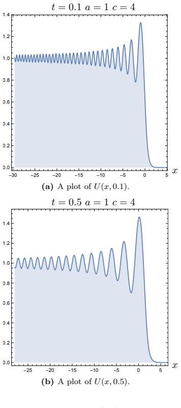
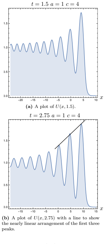
At $a=1$, $c=4$, solve the moving-interface problem (3)-(4) with an independent numerical method, such as a spectral or finite-difference scheme that enforces continuity of $q,q_x,q_{xx}$ at $x=0$, and compare with the plotted profiles at $t=0.1,0.5,1.5,2.75,4,8,20$: the reported growth of the maximum, the near-linear alignment of the first three peaks at $t=2.75$, and the approach to the stationary solution at $t=20$ are directly checkable. The representation in Proposition 3.1 can also be tested by substituting the integral expressions into the PDE and interface conditions.
Extended reading notes
Core claim
On its own terms, the paper's discovery is that the moving-interface linear problem $$u_t+u_{xxx}=-6a\,\mathbf{1}_{x<ct}\,u_x,\qquad u(x,0)=a\,\mathbf{1}_{x<0},$$ with continuity of $u,u_x,u_{xx}$ at $x=ct$, shares the short-time qualitative signatures of the KdV dispersive shock: growing oscillation amplitude, higher frequencies for larger $a$, and a transient near-linear arrangement of the leading peaks. The authors obtain the needed solution formula (Proposition 3.1) by adapting the unified transform method for interface problems, use it to compute high-accuracy profiles, and compare errors against the KdV solution computed by numerical inverse scattering. Their error measure shows the model dominates the naive linearization $F=0$ in the small-amplitude limit, with errors that decay in $|x|$. At long times the model tends to a stationary solution with oscillations on the left side of the front, which is not the KdV long-time behavior; the paper presents this difference explicitly as the boundary of the model's validity.
Load-bearing premise
All the plotted conclusions rest on the stated solution formula for the moving-interface problem, which the paper gives without proof; if that formula is not correct or the numerical evaluation of its integrals is not accurate at the times shown, the claimed reproduction of shock features is unsupported.
Editorial extensions
If this is right
- For step initial data, the linear model's maximum profile amplitude grows for small times, a signature the authors trace to the nonlinearity in KdV and show is preserved in the linear moving-interface model.
- Increasing the jump amplitude $a$ increases the frequency of the oscillations in the model, matching the amplitude-frequency relation of KdV dispersive shocks.
- After rescaling, the model is the universal small-amplitude limit for general initial data of the form $a(v(x)+h(x))$, so integrable corrections to the step contribute only lower-order effects.
- In the small-amplitude limit the error between the model and KdV is $O(a^{-1})$, with a smaller constant than for the naive linearization, and the error decays for large $|x|$.
- Because the model is faithful at short times but not at long times, comparisons of nonlinear PDE predictions with experiments should use sufficiently long times for the nonlinearity to manifest; the paper states this as a cautionary consequence.
Reading between the lines
- The same freezing recipe should transfer to other dispersive equations whose nonlinear term acts as a coefficient of $u_x$; replacing that coefficient by its left/right limiting values across a moving front should produce the same short-time oscillation growth.
- A practical extension is iterative re-linearization: solve the linear interface problem up to a positive time, linearize about that newer profile, and solve again; this could yield numerical schemes that track dispersion better, though it would require a fast multi-interface solver.
- Because the model reaches a stationary oscillatory state on the left at long times, an interesting test is whether a similar stationary pattern appears in KdV at intermediate times before solitons dominate; the paper does not pursue this.
Signed reviews
Editorial analysis
A structured set of objections, weighed in public.
Referee Report
Summary. The paper introduces a linear dispersive PDE with a moving-interface coefficient (equation (3)) that is intended to model early-time dispersive shock behavior of the Korteweg-de Vries equation with step-like initial data. The authors claim that, by linearizing about the step initial condition rather than about zero, the model reproduces several qualitative features of KdV dispersive shocks: growing oscillation amplitude, frequency increase with amplitude, transient linear peak arrangement, and a low-amplitude error smaller than that of the naive linearization. The model is solved formally using the unified transform method (UTM), leading to an explicit integral representation (Proposition 3.1). The paper compares this solution against numerics for KdV and against the stationary long-time limit, concluding that the linear model is a better short-time linearization than linearizing about zero while deviating at long times.
Significance. If the central claim is correct, the paper offers a conceptually interesting observation: a genuinely linear model with a simple moving interface can mimic several hallmarks of nonlinear dispersive shocks, which are usually regarded as intrinsically nonlinear phenomena. The idea of linearizing about the initial condition to obtain a piecewise-constant linear operator is suggestive and could be useful for cheap short-time estimates in other dispersive equations. The paper also includes explicit long-time asymptotics for the model and a comparison with a numerical KdV solver. However, the significance is currently conditional because the main supporting evidence is numerical and depends on an unproved solution representation, and the one free parameter (front speed c) is set to the known KdV shock speed in the comparisons.
major comments (4)
- [§3, Proposition 3.1] Proposition 3.1, which provides the explicit solution representation used for every figure in the paper, is stated without proof. The only justification is the sentence: 'The proof of this proposition may be obtained by following the method of [6], suitably modified in light of the results of [4].' Since all qualitative claims—oscillation growth, peak arrangement, and the error comparison in Figure 5—are computed from this representation, the central claim of the paper is unsupported unless this proposition is proved or at least verified independently. The authors should include a proof or a precise citation to a fully worked argument, and ideally an independent numerical check (e.g., direct time-stepping of the linear PDE (3)) for the plotted parameter values.
- [§4 and Figures 1–5] The numerical evaluation of the UTM integrals is not reproducible from the text. The paper states that the methodology 'is not asymptotically accurate' but does not specify the contour deformation, the quadrature rules, or the discretization parameters used to produce Figures 1–5. Without this information, the reader cannot assess whether the displayed oscillations, the transient peak alignment, or the error comparison are genuine properties of the model or numerical artifacts. The authors should provide full numerical details (contours, tolerance, number of quadrature points) or release code, and ideally compare with a direct numerical solution of (3) at a few (x,t) values.
- [§4.1] The short-time analysis is heuristic. The paper argues that analyzing U(x,t) = Q(x - gamma t, t) at fixed t for large c is equivalent to small time because of the scaling t -> c^{-3/2}t, but no rigorous asymptotic statement is made, and no error bounds are provided. Since the claim that the linear model is a 'better short-time linearization' is one of the central conclusions, the authors should either state a rigorous asymptotic result (with error estimates) or clearly label this as a numerical observation and support it with quantitative convergence data.
- [§2 and §4.4] The front speed c is introduced as a free parameter but is set to c = 4a in the comparisons with KdV, which is precisely the known speed of the KdV dispersive shock. This means the model is given the velocity of the phenomenon it is claimed to reproduce. The other qualitative features (oscillations, amplitude growth, peak arrangement) are not forced by this choice, so the issue is secondary, but it should be addressed explicitly: the authors should either justify c = 4a on independent grounds or demonstrate that the qualitative agreement is robust to variations in c over a range of values.
minor comments (4)
- [General] The paper contains several typos and minor notation inconsistencies, including 'In Figure 1a we plot' while the figure caption refers to 'A plot of U(x, 0.1)' with no subfigure label, and the use of 'ν' versus 'nu' in the displayed system for the functions g_j in Section 3. A careful proofreading is recommended.
- [§4.3] The stationary solution formulas in Section 4.3 are not fully derived; in particular, the constants c1, c2, b1, b2, b3 are stated without explanation. Adding a brief derivation or a reference would improve clarity.
- [§4.4] In the small-amplitude discussion, the error comparison in Figure 5 is presented only at a single time t = 0.1 and without error bars or convergence data. A short discussion of the dependence on t and on the numerical resolution of u_KdV would make the comparison more convincing.
- [§5] The concluding sentence 'Our results are not contingent on the unified transform method' is misleading: while the model itself is independent of UTM, every displayed solution and all numerical evidence in the paper rely on the UTM representation of Proposition 3.1. The authors should clarify that the qualitative conclusions are not contingent on UTM as a method, but the numerical verification is.
Circularity Check
The model's front speed c=4a is an input borrowed from KdV rather than a predicted output; the rest of the qualitative comparison is independent, so the circularity is partial.
-
fitted input called prediction
[Section 2 (model definition, eqs. (2)-(4)); Section 4.4 (comparison item 1); Section 1 (KdV shock speed).]
"Solutions to (1) with F (u;x,t ) = u(x,t ) are characterized by a dispersive shock wave that moves with velocity +4 a ... Here c is the front speed and is arbitrary. For example, c = 4a is an obvious choice to model the case F (u;x,t ) = u(x,t ). ... 1. u(x,t ) =u(x,t ;a, 4a), the solution of (3)."
The linear model is built around a moving interface x=ct, so its front speed equals the parameter c. The KdV comparison then fixes c=4a, which Section 1 identifies as the velocity of the KdV dispersive shock. The model is therefore given exactly the speed of the phenomenon it is said to reproduce; any agreement in front propagation is by construction rather than emergent. The other features (growing maximum amplitude, amplitude-dependent frequency, transient peak alignment) are not encoded by c=4a and are checked against an external KdV computation, so this step is only partially circular.
full rationale
The derivation of the linear model itself is explicit and not circular: F in (2) is a deliberate choice, and the moving-interface reduction to (4) is algebraic. The UTM representation in Proposition 3.1 is stated without proof ('The proof of this proposition may be obtained by following the method of [6], suitably modified in light of the results of [4]'), and all plotted q(x,t) values are computed from it; that is a verification gap, but it is not circularity, because [6] and [4] supply a method rather than assuming the present conclusions. The self-citations [2] and [4] are also not load-bearing in a circular sense: [2] provides an independent numerical KdV benchmark and [4] is a prior interface-method paper to which Proposition 3.1 defers. The only genuine input/output overlap is the front speed: c is free in the model and is set to 4a, the known KdV shock speed, before comparing. That makes the reproduced shock speed an input, not a prediction. However, the central qualitative claims and the Figure 5 error comparison have independent content and are not forced by c=4a, so a moderate partial-circularity score of 4 is appropriate rather than a higher score.
Assumptions & free parameters
free parameters (1)
- c (front speed) =
4a in KdV comparisons; otherwise free
assumptions (5)
- ad hoc to paper Proposition 3.1 gives the correct solution representation for (4).
- domain assumption Continuity of q, qx, and qxx across the moving interface x = ct is the correct interpretation of the piecewise-constant coefficient problem.
- ad hoc to paper Linearizing about the step initial condition, replacing F by the step value a behind the front and 0 ahead, yields a valid short-time approximation to KdV.
- domain assumption The KdV dispersive shock speed is 4a and solitons move faster than 4a, taken from [1,2].
- domain assumption For the long-time stationary analysis, c - 6a < 0 (equivalently gamma > 1/6) is assumed and gamma is kept fixed.
invented entities (1)
-
Piecewise-constant moving-interface linear model (3)
Cite this review
Pith. "Pith review of Linear Dispersive Shocks." pith.science (2026). https://pith.science/paper/5AZ5LI4P
@misc{pith2026190808716,
  author       = {Pith},
  title        = {Pith review of: Linear Dispersive Shocks},
  year         = {2026},
  howpublished = {\url{https://pith.science/paper/5AZ5LI4P}},
  note         = {Machine review of arXiv:1908.08716}
}
read the original abstract
We present a linear dispersive partial differential equation which manifests a number of qualitative features of dispersive shocks, typically thought to occur only in nonlinear models. The model captures much of the short time phenomenon but deviates from the full nonlinear model in its long time behavior. Though we limit our present discussion to dispersive shocks occurring in the Korteweg-de Vries equation, our work extends readily to other higher order dispersive models too.
Figures

Figures from the paper (2 more)


Reference graph
Works this paper leans on
-
[6]
N E Sheils and B Deconinck, Interface Problems for Dispersive Equations , Studies in Applied Mathematics 134 (2015), no. 3, 253–275. 12
work page 2015
-
[4]
B Deconinck, N E Sheils, and D A Smith, The Linear KdV Equation with an Interface , Communications in Mathematical Physics 347 (2016), no. 2, 489–509
work page 2016
- [1]
-
[2]
D Bilman and T Trogdon, On numerical inverse scattering for the Korteweg-de Vries equation with discontinuous step-like data , arXiv preprint arXiv:1809.09263 (2018). 11
work page Pith review arXiv 2018
-
[3]
G Biondini and T Trogdon, Gibbs Phenomenon for Dispersive PDEs on the Line, SIAM Journal on Applied Mathematics 77 (2017), no. 3, 813–837
work page 2017
-
[5]
I Egorova, Z Gladka, V Kotlyarov, and G Teschl, Long-time asymptotics for the Korteweg–de Vries equation with step-like initial data , Nonlinearity 26 (2013), no. 7, 1839–1864
work page 2013
Reviewed August 14, 2026 · model on record in the stance chip above.
Discussion (0). Continue with ORCID to comment.