REVIEW 3 major objections 4 minor 60 references
Adjoint-based Recovery of Thermal Fields from Displacement or Strain Measurements
T0 review · 3 major / 4 minor · reviewed 2026-08-12 · deepseek-v4-flash
Pith's one-line read Using only displacement or strain measurements, a finite-element adjoint optimizer reconstructs the structure's temperature field, and the sensors do not need to be inside the heated region.
desk verdict A useful engineering application of standard adjoint inversion, but the paper has a serious unresolved discrepancy between the printed thermal-stress equations and the two tested element types, plus an inverse-crime validation. read the letter →
The pith
A machine-rendered reading of the paper's core claim, the machinery that carries it, and where it could break.
The reading
What carries the argument
The central object is the Lagrangian functional $\mathcal{L}(u,\Delta T,\tilde{u}) = I(u,\Delta T) + \tilde{u}^t (f_{\mathrm{ext}} + f_{\Delta T} - K u)$, which couples the measurement mismatch $I$ to the finite-element equilibrium equations. The stationarity conditions produce the forward problem $K u = f_{\mathrm{ext}} + f_{\Delta T}$, the adjoint problem $K^t \tilde{u} = \frac{\partial I}{\partial u}$ (with $K^t = K$ for structural systems), and the gradient formula for the thermal field. Vertex Morphing acts as the regularizer: a kernel operator maps physical nodal temperatures through a control field, smoothing the gradient and suppressing high-frequency artifacts in the ill-posed inversion.
What would settle it
Run the same inversion on a physical plate-with-a-hole specimen where the heated patch is known and measured with thermocouples, but feed the optimizer only strain-gauge readings that include realistic noise and unknown small load variations; if the recovered peak temperature stays far below the true value, the heated region is misplaced, or the root-mean-square error no longer beats kriging, the central claim fails.
Extended reading notes
Core claim
The central claim is that the inverse problem of thermal field identification is tractable from displacement or strain data alone: given the load cases and the sensor readings, minimizing the weighted mismatch between measured and computed displacements yields a spatial temperature distribution that approximates the target field. The derivation shows that the gradient of the cost function with respect to the nodal temperature changes requires only the forward solve and an adjoint solve with the same stiffness matrix, since the stiffness matrix is symmetric for these structural systems, and the gradient takes the form $\nabla I(\Delta T) = \frac{\partial I}{\partial \Delta T} + \tilde{u}^t \frac{\partial f_{\Delta T}}{\partial \Delta T}$.
Load-bearing premise
The demonstrations assume the displacement data come from the same noiseless linear finite-element model used in the inversion, with the loads, boundary conditions, and material properties known exactly.
Editorial extensions
If this is right
- Thermal fields can be reconstructed by deformation sensors alone, reducing reliance on temperature sensors in inaccessible or non-uniformly heated regions.
- Sensor placement does not need to intersect the heated region; it only needs to be sensitive to the deformation that region produces.
- Increasing sensor count and improving sensor placement sharpens both the magnitude and the localization of the recovered temperature field.
- Vertex Morphing filtering consistently lowers reconstruction error, with root-mean-square error reductions of up to 16%, 24.4%, and 18% across the three examples.
- At equal sensor counts, the proposed physics-based approach beats k-nearest-neighbor and kriging interpolation, with root-mean-square error reductions of up to 38.4%, 94%, and 40%.
Reading between the lines
- Inference: the method's success likely depends on the accuracy of the finite-element model and on the assumption that the measured deformation is purely thermal-mechanical; realistic sensor noise, load uncertainty, and model error are listed by the authors as future work and would probably degrade the reconstruction.
- Inference: combining displacement or strain sensors with temperature sensors in the same cost function could fill the low-sensitivity 'blind spots' the paper observes near corners and edges.
- Inference: since thermal loads enter the equilibrium equations as equivalent nodal forces through $f_{\Delta T}$, the same adjoint machinery could be redirected to identify other distributed quantities, such as prestress or spatially varying material properties.
- Inference: extending the cost function over time would allow recovery of transient thermal fields, at the cost of solving many more forward and adjoint problems.
Editorial analysis
A structured set of objections, weighed in public.
Referee Report
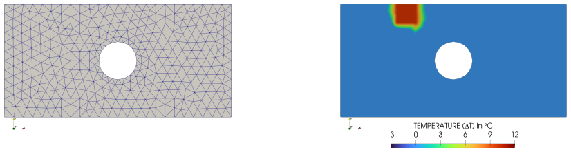
Summary. The paper proposes a finite-element adjoint-based optimization procedure to reconstruct spatial temperature fields from displacement or strain measurements under known loads. The method models thermal strains as equivalent nodal loads, derives the adjoint gradient of a weighted least-squares misfit, and regularizes the ill-posed nodal temperature update with Vertex Morphing filtering. Three numerical examples are presented: a plate with a hole modeled with plane-stress triangles, a truss bridge, and a simplified Hoover Dam modeled with tetrahedra. In each case, a target temperature field is prescribed, displacement/strain data are generated synthetically, and the optimizer attempts to recover the field from sensor measurements. The results are compared with k-nearest-neighbor, ordinary kriging, and universal kriging interpolations using temperature sensors in identical configurations, with reported RMSE reductions up to 38.4%, 94%, and 40% for the three examples.
Significance. If the claims are borne out, the method would be a useful addition to structural health monitoring and digital twin workflows, since it would allow thermal fields to be reconstructed from deformation sensors alone, including scenarios where no temperature sensor is located in the heated region. The paper is clearly written and the optimization machinery is standard; the comparison with spatial interpolation methods is informative, and the authors are explicit about many limitations (e.g., noise, parameter uncertainty, sensor blind spots) in Section 5. The main concerns are that the printed thermal-load equations do not match the element types tested in Examples 1 and 2, and that the numerical validation uses an inverse-crime setup with noiseless synthetic data, so the stated claim of 'accurate reconstruction' is stronger than the evidence supports. These issues are fixable and do not invalidate the underlying idea.
major comments (3)
- [Section 3.1, Eqs. (3) and (7)] Equation (3) gives sigma_ij = -alpha E/(1-2nu) Delta T delta_ij, which is the triaxially constrained 3D thermal stress, after the text introduces the equation as the thermal stress for a 'one-dimensional rod'. The uniaxial rod stress would be -alpha E Delta T. The same coefficient is carried into the finite-element thermal nodal load in Eq. (7). This is inconsistent with the examples: Section 4.1 uses plane-stress triangular elements, where the correct thermal nodal-load coefficient is alpha E/(1-nu), and Section 4.2 uses truss elements, where the axial coefficient is alpha E. Only the tetrahedral dam example of Section 4.3 matches the printed E/(1-2nu) coefficient. Since the paper describes an 'FE-method-dependent' procedure and all simulations were run in Kratos, Eqs. (3)-(7) should describe the implemented model; as printed, they do not, so a reader cannot reproduce the reported reconstructions from the paper. Please correct the equations or state clearly how the thermal-load coefficient is adapted for each element formulation.
- [Section 4, opening; Section 5] All 'measured' data are generated by the same noiseless linear finite-element model that is used for the inversion, with perfectly known external loads, boundary conditions, and material properties. This is an inverse-crime setup. The abstract's conclusion that the approach 'can accurately reconstruct the target thermal distribution' is therefore not established for realistic measurements containing sensor noise, load uncertainty, or model error; these effects are listed as future work in Section 5. Please either add numerical experiments with additive sensor noise, perturbed material/load parameters, or a mismatched mesh/model, or qualify the central claim so that it is limited to the noiseless synthetic setting.
- [Section 4.4.3, Tables 1-3] The headline RMSE reductions (up to 38.4%, 94%, and 40%) compare the proposed displacement-based adjoint method with interpolation methods that use temperature sensors only. In configurations where no temperature sensor detects the heated region (e.g., the 6-sensor plate case in Figure 21a), the interpolation baseline returns essentially Delta T = 0 by construction, so large percentage improvements are expected and do not indicate superiority in a like-for-like information setup. The comparison is still meaningful for the claimed 'sensors not in the region of interest' scenario, but the abstract and Section 4.4.3 should state this asymmetry explicitly rather than presenting the percentages as a general accuracy comparison between reconstruction methods.
minor comments (4)
- [Section 3.2, Eq. (8)] The strain misfit term in Eq. (8) uses the notation ums_ij, but the text defines the measured strain as sms_ij; please make the notation consistent.
- [After Eq. (12)] The symbol Js_ij is introduced to denote the displacement-strain relationship, but the cost function in Eq. (8) uses Is_ij; please align or define both symbols.
- [Section 4.1] The Young's modulus for the plate is given as E = 2e12 Pa, which is an order of magnitude above typical structural steel; if this value is intentional, please state so, otherwise it appears to be a typo.
- [Tables 1-3] Several table captions refer to a single figure number (e.g., Table 2 refers to 'Figure 8') when the target distribution is only the bottom half of the displayed figure; please make the cross-references more precise.
Circularity Check
No significant circularity: the adjoint recovery of the thermal field is validated against externally prescribed target distributions, and the self-citations present are not load-bearing.
full rationale
The central derivation chain is not circular. The forward problem (Eqs. 7 and 9a) maps a nodal temperature field to displacements through the thermal load vector and stiffness matrix; the cost function (Eq. 8) compares computed displacements or strains with measured values; and the adjoint gradient (Eqs. 13-15) is derived explicitly from the Lagrangian (Eq. 11) within the paper itself, so no step of the derivation is defined in terms of the predicted quantity. The validation is against externally prescribed target fields (Section 4), with RMSE tables (Section 4.4.3) computed against those targets; no parameter is fitted to the target to make the reconstruction succeed, since the Barzilai-Borwein step (Eq. 16) and the Vertex Morphing radius are chosen a priori and results are reported both with and without filtering (e.g., Figures 5, 11, 17). Self-citations (Antil et al. 2018 for the Lagrangian functional; Antonau 2023 for the BB method; Antonau et al. 2022 and Hojjat et al. 2014 for Vertex Morphing; Airaudo, Lohner, and Warnakulasuriya et al. for the analogous weakness-identification approach) are present but not load-bearing: the Lagrangian derivation is reproduced in full, the BB update is stated explicitly, and Vertex Morphing is shown to be a smoothing convenience rather than a requirement for reconstruction. Two genuine caveats belong to correctness and validity risk rather than circularity. First, the displacement measurements are synthetic, generated by the same finite-element model used for the inversion, which is an inverse-crime consistency test with noiseless data; the paper itself lists sensor noise, parameter uncertainty, and time lag as open future-work items in Section 5, and that limitation is weighed here as a modeling caveat, not as a logical reduction of the prediction to its inputs. Second, the printed thermal-stress coefficient alpha*E/(1-2*nu) in Eqs. (3) and (7) matches the 3D tetrahedral dam example but is inconsistent with the plane-stress plate (alpha*E/(1-nu)) and truss bridge (alpha*E) elements used in Sections 4.1 and 4.2, which is a reproducibility gap between the stated equations and the tested Kratos models; again, this concerns whether the paper describes the model it ran, not whether the recovered fields reduce to their inputs.
Assumptions & free parameters
free parameters (6)
- Vertex Morphing filter radius r =
5 (Plate), 6 (Bridge), 50 (Dam)
- Maximum gradient-descent stepsize =
2.5e-3 (Plate), 2.5e-2 (Bridge), 1e-1 (Dam)
- Convergence criterion =
1e-5 times initial cost function
- Cost function weights w_md and w_ms =
unspecified (assumed equal)
- kNN hyperparameters =
k=3 (Plate/Bridge), k=5 (Dam), inverse distance weighting
- Kriging variogram and trend =
Gaussian variogram, regional linear trend for universal kriging
assumptions (4)
- domain assumption Linear isotropic thermoelasticity with constant Young's modulus (Eqs. 2-5, Section 3.1).
- domain assumption The finite element model is an exact representation of the physical structure, including known external loads and boundary conditions (Eq. 9, Section 4).
- standard math The reduced optimization problem is convex enough for steepest descent to reach a meaningful minimum (Section 3.3).
- ad hoc to paper Smoothness imposed by Vertex Morphing is an appropriate prior for the unknown temperature field (Section 3.3.1).
Cite this review
Pith. "Pith review of Adjoint-based Recovery of Thermal Fields from Displacement or Strain Measurements." pith.science (2026). https://pith.science/paper/5FA5LYNF
@misc{pith2026241118118,
  author       = {Pith},
  title        = {Pith review of: Adjoint-based Recovery of Thermal Fields from Displacement or Strain Measurements},
  year         = {2026},
  howpublished = {\url{https://pith.science/paper/5FA5LYNF}},
  note         = {Machine review of arXiv:2411.18118}
}
read the original abstract
A finite-element method dependant adjoint-based procedure to determine the temperature field of structures based on measured displacements or strains and a set of standard loads is developed and tested. Given a series of force and deformation measurements, the temperature field is obtained by minimizing the adequately weighted differences between the measured and computed values. Three numerical examples - a Plate With a Hole, a Bridge, and a Hoover Dam example - each with multiple sensors distributed in different configurations, demonstrate the procedure's capabilities. A target temperature distribution is prescribed in all cases, and the displacement sensor data is recorded. The optimization algorithm (here, steepest descent with Barzilai-Borwein step) uses this data to optimize the temperatures such that the same deformation is obtained at the sensor locations. Vertex Morphing is used as a filter to mitigate the ill-conditioning. Results show that the proposed approach can accurately reconstruct the target thermal distribution, especially when more sensors are used. Additionally, it is observed that the sensors do not need to be positioned in the region of interest; the method remains effective as long as the sensors can detect changes related to that area. A comparison with standard spatial interpolation techniques, namely, k-nearest neighbors and ordinary and universal kriging, is performed using temperature sensors in the same configurations. The proposed approach performs remarkably better than the interpolation techniques with a reduction in the root-mean-squared error of up to 38.4%, 94%, and 40%, for the Plate With a Hole, the Bridge, and the Dam examples, respectively.
Figures

Figures from the paper (26 more)


Reference graph
Works this paper leans on
-
[9]
Antonau, I., Warnakulasuriya, S., Bletzinger, K.U., Bluhm, F.M., Hojjat, M., Wüchner, R.,
Formulation and regularization of the optimization problem for adjoint-based digital twin construction, in: ECCOMAS Congress 2024: 9th European Congress on Computational Methods in Applied Sciences and Engineering, Lisbon, Portugal. Antonau, I., Warnakulasuriya, S., Bletzinger, K.U., Bluhm, F.M., Hojjat, M., Wüchner, R.,
work page 2024
-
[11]
Journal of Constructional Steel Research 142, 31–43
Experimental and numerical study on temperature distribution of square hollow section joints. Journal of Constructional Steel Research 142, 31–43. DOI: https: //doi.org/10.1016/j.jcsr.2017.12.006. Bayraktar, A., Akköse, M., Ta¸ s, Y., Erdi¸ s, A., Kur¸ sun, A.,
-
[12]
Journal of Civil Structural Health Monitoring 12, 833–844
Long-term strain behavior of in-service cable- stayed bridges under temperature variations. Journal of Civil Structural Health Monitoring 12, 833–844. DOI:https://doi.org/10.1007/s13349-022-00578-0 . Bui, K.A., Sancharoen, P ., Tanapornraweekit, G., Tangtermsirikul, S., Nanakorn, P .,
-
[13]
Engineering Structures 174, 165–177
FEA model for the simulation of the hydration process and temperature evolution during the concreting of an arch dam. Engineering Structures 174, 165–177. DOI:https://doi.org/10.1016/j.engstruct.2018.07.065. 36/40 Chen, H., Liu, Z.,
-
[15]
Engineering Structures 253, 113783
A data-driven approach for drive-by damage detection in bridges considering the influence of temperature change. Engineering Structures 253, 113783. DOI: https://doi. org/10.1016/j.engstruct.2021.113783. Dadvand, P ., Rossi, R., Oñate, E.,
arXiv 2021
-
[17]
An efficient model for simulation of temperature field of steel-concrete composite beam bridges. Structures 43, 1868–1880. DOI: https://doi.org/10.1016/j.istruc.2022. 05.079. Ferrándiz, V .M., Bucher, P ., Zorrilla, R., Warnakulasuriya, S., Rossi, R., Cornejo, A., jcotela, Roig, C., Maria, J., tteschemacher, Masó, M., Casas, G., Núñez, M., Dadvand, P ., L...
-
[18]
DOI:https://doi.org/10.5281/zenodo.6926179
Kratosmultiphysics/kratos: Release v9.5. DOI:https://doi.org/10.5281/zenodo.6926179. Fletcher, R.,
-
[22]
Kromanis, R., Kripakaran, P .,
DOI: https: //doi.org/10.1061/(asce)be.1943-5592.0001085. Kromanis, R., Kripakaran, P .,
Show all 60 references
-
[24]
Hojjat, M., Stavropoulou, E., Bletzinger, K.U.,
DOI: https://doi.org/10.1061/ (asce)be.1943-5592.0001454. Hojjat, M., Stavropoulou, E., Bletzinger, K.U.,
1943
-
[25]
Journal of Civil Structural Health Monitoring 6, 545–560
Damage detection of a highway bridge under severe temperature changes using extended kalman filter trained neural network. Journal of Civil Structural Health Monitoring 6, 545–560. DOI: https://doi.org/10.1007/s13349-016-0173-8 . Jin, C., Li, J., Jang, S., Sun, X., Christenson, R.,
-
[26]
1943-5592.0001708
DOI: https://doi.org/10.1061/(asce)be. 1943-5592.0001708. Sheng, X., Zhou, T., Huang, S., Cai, C., Shi, T.,
1943
-
[27]
Applied Thermal Engineering 30, 2146–2156
Practical procedure for predicting non-uniform temperature on the exposed face of arch dams. Applied Thermal Engineering 30, 2146–2156. DOI: https://doi.org/10. 1016/j.applthermaleng.2010.05.027. 37/40 Kosti´ c, B., Gül, M.,
2010
-
[30]
Antil, H., Kouri, D.P ., Lacasse, M.D., Ridzal, D
DOI: https://doi.org/10.1002/nla.2481. Antil, H., Kouri, D.P ., Lacasse, M.D., Ridzal, D. (Eds.),
-
[32]
Advances in Structural Engineering 15, 447–459
Analysis of thermal environmental effects on precast, prestressed concrete bridge girders: temperature differentials and thermal deformations. Advances in Structural Engineering 15, 447–459. DOI:https://doi.org/10.1260/1369-4332.15.3.447. Lin, P ., Peng, H., Fan, Q., Xiang, Y....
-
[33]
KSCE Journal of Civil Engineering 25, 1326–1340
A 3D thermal field restructuring method for concrete dams based on real-time temperature monitoring. KSCE Journal of Civil Engineering 25, 1326–1340. DOI:https://doi.org/10.1007/s12205-021-1084-8 . Liu, X., Zhang, C., Chang, X., Zhou, W., Cheng, Y., Duan, Y.,
-
[34]
Applied Thermal Engineering 78, 449–459
Precise simulation analysis of the thermal field in mass concrete with a pipe water cooling system. Applied Thermal Engineering 78, 449–459. DOI: https: //doi.org/10.1016/j.applthermaleng.2014.12.050. Lohner, R., Airaudo, F., Antil, H., Wüchner, R., Meister, F., Warnakulasuriy...
2014 doi
-
[36]
Damage detection in civil engineering structure considering temperature effect, in: Dynamics of Civil Structures, Volume 4: Proceedings of the 32nd IMAC, A Conference and Exposition on Structural Dynamics, 2014, Springer. pp. 187–196. DOI:https://doi.org/ 10.1007/978-3-319-045...
2014 doi
-
[37]
Engineering Structures 127, 700–718
Static load testing with temperature compensation for structural health monitoring of bridges. Engineering Structures 127, 700–718. DOI: https://doi.org/10. 1016/j.engstruct.2016.09.018. Pan, J., Liu, W., Wang, J., Jin, F., Chi, F.,
2016
-
[38]
Measurement 188, 110585
A novel reconstruction method of temperature field for thermomechanical stress analysis of arch dams. Measurement 188, 110585. DOI: https://doi.org/10. 1016/j.measurement.2021.110585. Peeters, B., Maeck, J., De Roeck, G.,
2021
-
[39]
Frontiers in Materials 7, 587738
A positioning method of temperature sensors for monitoring dam global thermal field. Frontiers in Materials 7, 587738. DOI: https://doi.org/ 10.3389/fmats.2020.587738. Potgieter, I.C.,
2020
-
[40]
Structural Health Monitoring 13, 82–93
Output-only structural health monitoring in changing envi- ronmental conditions by means of nonlinear system identification. Structural Health Monitoring 13, 82–93. DOI:https://doi.org/10.1177/1475921713502836. Roberts-Wollman, C.L., Breen, J.E., Cawrse, J.,
-
[42]
Applied Thermal Engineering 85, 160–171
A new 1D analytical model for computing the thermal field of concrete dams due to the environmental actions. Applied Thermal Engineering 85, 160–171. DOI: https: //doi.org/10.1016/j.applthermaleng.2015.04.023. Sharma, S., Sen, S.,
2015 doi
-
[44]
Case Studies in Construction Materials 16, e01026
Prediction of vertical temperature gradient on concrete box-girder considering different locations in china. Case Studies in Construction Materials 16, e01026. DOI:https://doi.org/10.1016/j.cscm.2022.e01026. Soo Lon Wah, W., Chen, Y.T.,
2022 doi
-
[45]
Journal of Low Frequency Noise, Vibration and Active Control 39, 572–587
A new approach toward damage localization and quantification of structures under changing temperature condition. Journal of Low Frequency Noise, Vibration and Active Control 39, 572–587. DOI: https://doi.org/10.1177/1461348418793079. Sun, L., Zhang, W., Nagarajaiah, S.,
-
[46]
Journal of Bridge Engineering 24, 04018111
Bridge real-time damage identification method using inclination and strain measurements in the presence of temperature variation. Journal of Bridge Engineering 24, 04018111. DOI:https://doi.org/10.1061/(asce)be.1943-5592.0001325. Tong, M., Tham, L., Au, F., Lee, P .,
1943
-
[48]
Wang, S., Chai, B., Liu, Y., Gu, H.,
(Accessed online on 28/10/2024). Wang, S., Chai, B., Liu, Y., Gu, H.,
2024
-
[51]
Yang, X.P ., Chang, X.L., Liu, X.H.,
Optimal sensor placement methodology for adjoint-based weakening localization in structures, in: ECCOMAS Congress 2024: 9th European Congress on Computational Methods in Applied Sciences and Engineering, Lisbon, Portugal. Yang, X.P ., Chang, X.L., Liu, X.H.,
2024
-
[52]
Applied Mechanics and Materials 212, 887–890
FEM simulation of temperature and thermal stress of xiaowan arch dam. Applied Mechanics and Materials 212, 887–890. DOI: https://doi.org/10.4028/www.scientific. net/amm.212-213.887. Zhang, H., Gül, M., Kosti´ c, B.,
-
[53]
Zhang, W.m., Zhang, Z.h., Wang, Z.w., Chen, B.,
DOI:https://doi.org/10.1061/(asce)as.1943-5525.0000987. Zhang, W.m., Zhang, Z.h., Wang, Z.w., Chen, B.,
1943
-
[54]
Engineering Structures 315, 118476
Temperature analysis and prediction for road-rail steel truss cable-stayed bridges based on the structural health monitoring. Engineering Structures 315, 118476. DOI:https://doi.org/10.1016/j.engstruct.2024.118476. Zheng, D., Du, Z.K., Peng, S.C.,
2024
-
[55]
Simulation of two-dimensional temperature field via kriging method based on limited conditioning points in an arc dam, in: IOP Conference Series: Earth and Environmental Science, IOP Publishing. p. 032058. DOI: https://doi.org/10.1088/1755-1315/304/3/032058. Zhong, R., Hou, G....
-
[56]
Applied Thermal Engineering 124, 1409–1417
An improved composite element method for the simulation of temperature field in massive concrete with embedded cooling pipe. Applied Thermal Engineering 124, 1409–1417. DOI:https://doi.org/10.1016/j.applthermaleng.2017.06.124. 39/40 Zhou, G.D., Yi, T.H.,
2017 doi
-
[57]
International Journal of Distributed Sensor Networks 9, 217983
Thermal load in large-scale bridges: a state-of-the-art review. International Journal of Distributed Sensor Networks 9, 217983. DOI: https://doi.org/10.1155/2013/217983. Zhou, G.D., Yi, T.H.,
2013 doi
-
[58]
1016/j.istruc.2023.105568
DOI: https://doi.org/10. 1016/j.istruc.2023.105568. Wang, X., Gao, Q., Liu, Y.,
2023
-
[59]
Mathematical Problems in Engineering 2014, 1–19
A summary review of correlations between temperatures and vibration properties of long-span bridges. Mathematical Problems in Engineering 2014, 1–19. DOI: https://doi.org/10.1155/ 2014/638209. Zhou, H., Pan, Z., Liang, Z., Zhao, C., Zhou, Y., Wang, F.,
2014
-
[60]
KSCE Journal of Civil Engineering 23, 1911–1922
Temperature field reconstruction of concrete dams based on distributed optical fiber monitoring data. KSCE Journal of Civil Engineering 23, 1911–1922. DOI:https://doi.org/10.1007/s12205-019-0787-6 . Zhouc, H., Zhou, Y., Zhao, C., Liang, Z.,
1911 doi
-
[61]
Zuo, Z., Hu, Y., Li, Q., Liu, G.,
DOI: https://doi.org/10.14311/cej.2016.03.0014. Zuo, Z., Hu, Y., Li, Q., Liu, G.,
2016 doi
-
[62]
Finite Elements in Analysis and Design 102, 52–64
An extended finite element method for pipe-embedded plane thermal analysis. Finite Elements in Analysis and Design 102, 52–64. DOI: https://doi.org/10.1016/j.finel. 2015.05.002. 40/40
2015 doi
-
[198]
B ˛ aczkiewicz, J., Malaska, M., Pajunen, S., Heinisuo, M.,
DOI: https://doi.org/10.1007/s00158-022-03279-w . B ˛ aczkiewicz, J., Malaska, M., Pajunen, S., Heinisuo, M.,
-
[2001]
Computers & Structures 79, 583–593
Numerical modelling for temperature distribution in steel bridges. Computers & Structures 79, 583–593. DOI:https://doi.org/10.1016/s0045-7949(00)00161-9. Waka Kotahi NZ Transport Agency,
-
[2002]
Journal of Bridge Engineering 7, 166–174
Measurements of thermal gradients and their effects on segmental concrete bridge. Journal of Bridge Engineering 7, 166–174. DOI: https://doi.org/10.1061/ (asce)1084-0702(2002)7:3(166). Santillán, D., Salete, E., Toledo, M.,
2002
-
[2005]
On the barzilai-borwein method, in: Optimization and Control with Applications, Springer. pp. 235–256. DOI: https://doi.org/10.1007/0-387-24255-4_10 . Ghantasala, A., Najian Asl, R., Geiser, A., Brodie, A., Papoutsis, E., Bletzinger, K.U.,
-
[2010]
Archives of computational methods in engineering 17, 253–297
An object-oriented environment for developing finite element codes for multi-disciplinary applications. Archives of computational methods in engineering 17, 253–297. DOI: https: //doi.org/10.1007/s11831-010-9045-2 . Fan, J.S., Li, B.L., Liu, C., Liu, Y.F.,
-
[2012]
Engineering Structures 40, 20–38
Structural health monitoring of continuous prestressed concrete bridges using ambient thermal responses. Engineering Structures 40, 20–38. DOI: https://doi.org/10.1016/j. engstruct.2012.02.001. Lee, J.H., Kalkan, I.,
2012 doi
-
[2013]
Advanced Engineering Informatics 27, 486–495
Support vector regression for anomaly detection from measurement histories. Advanced Engineering Informatics 27, 486–495. DOI: https://doi.org/10.1016/j.aei. 2013.03.002. Kromanis, R., Kripakaran, P .,
2013 doi
-
[2014]
Computer Methods in Applied Mechanics and Engineering 268, 494–513
The Vertex Morphing method for node-based shape optimization. Computer Methods in Applied Mechanics and Engineering 268, 494–513. DOI: https://doi. org/10.1016/j.cma.2013.10.015. Hou, C., Chai, D., Cheng, H., Ning, S., Yang, B., Zhou, Y.,
2013 doi
-
[2015]
Structural damage detection for in-service highway bridge under operational and environmental variability, in: Sensors and Smart Structures Technologies for Civil, Mechanical, and Aerospace Systems 2015, SPIE. pp. 943–952. DOI: https://doi.org/10.1117/12. 2084384. Jin, F., Che...
2015 doi
-
[2016]
Construction and Building Materials 106, 523–532
Experimental analysis of temperature gradients in concrete box-girders. Construction and Building Materials 106, 523–532. DOI:https://doi.org/10.1016/j.conbuildmat. 2015.12.144. Abid, S.R., Xue, J., Liu, J., Tay¸ si, N., Liu, Y., Özakça, M., Briseghella, B.,
2015 doi
-
[2017]
Structural Control and Health Monitoring 24, e1998
Damage detection under varying temperature using artificial neural networks. Structural Control and Health Monitoring 24, e1998. DOI:https://doi.org/10.1002/stc.1998. Hagedorn, R., Martí-Vargas, J.R., Dang, C.N., Hale, W.M., Floyd, R.W.,
1998 doi
-
[2018]
volume 163 of The IMA Volumes in Mathematics and its Applications
Frontiers in PDE-constrained optimization. volume 163 of The IMA Volumes in Mathematics and its Applications. Springer, New York. ISBN: 978-1-4939-8635-4; 978- 1-4939-8636-1, DOI:https://doi.org/10.1007/978-1-4939-8636-1 . Papers based on the workshop held at the Institute for...
-
[2019]
Journal of Thermal Analysis and Calorimetry 135, 2019–2029
Temperature control and thermal-induced stress field analysis of GongGuoQiao RCC dam. Journal of Thermal Analysis and Calorimetry 135, 2019–2029. DOI: https://doi.org/10.1007/ s10973-018-7450-1 . Corbally, R., Malekjafarian, A.,
2019
-
[2020]
LRFD Bridge Design Specifications. 9th ed. Washington, DC. ISBN: 1560517387. ISBN (Online): 9781560517382, URL:https://aashtojournal. transportation.org/aashto-issues-updated-lrfd-bridge-design-guide/ . (Accessed on- line on 28/10/2024). Antil, H.,
2024
-
[2021]
Journal of Optimization Theory and Applications 189, 164–189
Realization of a frame- work for simulation-based large-scale shape optimization using vertex morphing. Journal of Optimization Theory and Applications 189, 164–189. DOI: https://doi.org/10.1007/s10957-021-01826-x . Glashier, T., Kromanis, R., Buchanan, C., 2024a. An iterative...
-
[2022]
Temperatures and gradients in concrete bridges: Experimental, finite element analysis and design, in: Structures, Elsevier. pp. 960–976. DOI:https://doi.org/10.1016/j.istruc.2022.01.070. Airaudo, F., Antil, H., Löhner, R., Rakhimov, U., 2024a. On the use of risk measures in di...
2022 doi
-
[2023]
Computer Methods in Applied Mechanics and Engineering 417, 116471
Adjoint-based determination of weaknesses in structures. Computer Methods in Applied Mechanics and Engineering 417, 116471. DOI: https://doi.org/10. 1016/j.cma.2023.116471. American Association of State Highway and Transportation Officials,
2023
-
[2024]
URL: https://arxiv.org/abs/ 2402.10326, arXiv:2402.10326
Mathematical opportunities in digital twins (math-dt). URL: https://arxiv.org/abs/ 2402.10326, arXiv:2402.10326. Antil, H., Dolgov, S., Onwunta, A.,
-
[2621]
Lohner, R., Airaudo, F., Antil, H., Wüchner, R., Meister, F., Warnakulasuriya, S., 2024b
DOI: https: //doi.org/10.2514/6.2024-2621. Lohner, R., Airaudo, F., Antil, H., Wüchner, R., Meister, F., Warnakulasuriya, S., 2024b. High-fidelity digital twins: Detecting and localizing weaknesses in structures. International Journal for Numerical Methods in Engineering (IJNM...
2024 doi
-
[2622]
Airaudo, F., Antil, H., Löhner, R., Warnakulasuriya, S., Antonau, I., Wüchner, R., 2024b
DOI:http://dx.doi.org/10.2514/6.2024-2622. Airaudo, F., Antil, H., Löhner, R., Warnakulasuriya, S., Antonau, I., Wüchner, R., 2024b. On the use of risk measures in digital twins to identify weaknesses in structures, in: ECCOMAS Congress 2024: 9th European Congress on Computati...
2024 doi
-
[3999]
Warnakulasuriya, S., Antonau, I., Airaudo, F., Löhner, R., Antil, H., Wüchner, R.,
DOI: https://doi.org/10.3390/s20143999. Warnakulasuriya, S., Antonau, I., Airaudo, F., Löhner, R., Antil, H., Wüchner, R.,
-
[4028]
Jin, C., Jang, S., Sun, X., Li, J., Christenson, R.,
DOI:https://doi.org/10.3390/w14244028. Jin, C., Jang, S., Sun, X., Li, J., Christenson, R.,
Reviewed August 12, 2026 · model on record in the stance chip above.
Discussion (0). Continue with ORCID to comment.