Adjoint Method versus Physics-Informed Neural Networks in PDE-Constrained Inverse Problems
Pith reviewed 2026-06-27 08:57 UTC · model grok-4.3
The pith
The representation of the unknown largely determines whether adjoint methods or PINNs perform better in PDE-constrained inverse problems.
A machine-rendered reading of the paper's core claim, the machinery that carries it, and where it could break.
Core claim
From a common abstract formulation the authors instantiate both methods on identical domains, governing equations, observation models, and regularization terms while matching the optimizer, unknown parameterization, and arithmetic precision. The results show that the representation of the unknown largely determines the preferred method: grid-based fields favor the discrete adjoint, whereas neural representations are native to PINNs and relevant for closure and constitutive modeling. For time-dependent problems, adjoint inversion can be dominated by trajectory storage and differentiation, while PINNs provide satisfactory reconstructions at lower cost. A PINN-warm-started adjoint strategy then
What carries the argument
The fair comparison protocol that enforces identical domains, governing equations, observation models, regularization terms, optimizer, unknown parameterization, and arithmetic precision to isolate the effect of unknown representation.
If this is right
- Grid-based fields make the discrete adjoint the stronger choice.
- Neural representations make PINNs the natural fit for closure and constitutive modeling tasks.
- Time-dependent problems favor PINNs when trajectory storage dominates adjoint cost.
- A PINN-warm-started adjoint recovers full adjoint accuracy at lower overall cost.
Where Pith is reading between the lines
- Hybrid strategies may become standard when the unknown mixes grid and neural elements.
- The cost advantage of PINNs in evolutionary problems could extend to other time-dependent systems such as reaction-diffusion or fluid-structure interaction.
- Future work could test whether the representation preference persists when the unknown must satisfy additional physical constraints such as positivity or monotonicity.
Load-bearing premise
That the matched settings and four chosen benchmarks produce a comparison whose outcomes generalize beyond those specific cases.
What would settle it
A new benchmark in which a grid-based unknown is inverted and the PINN version outperforms the adjoint version, or vice versa, under the same matched protocol.
Figures
read the original abstract
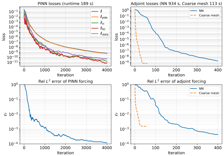
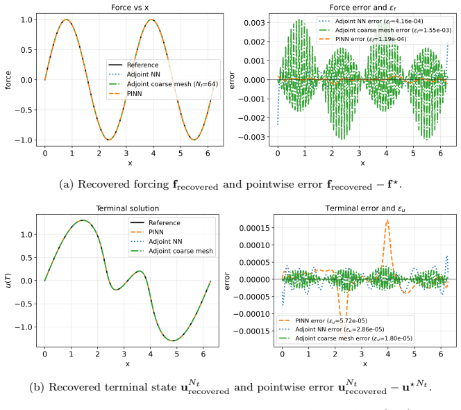
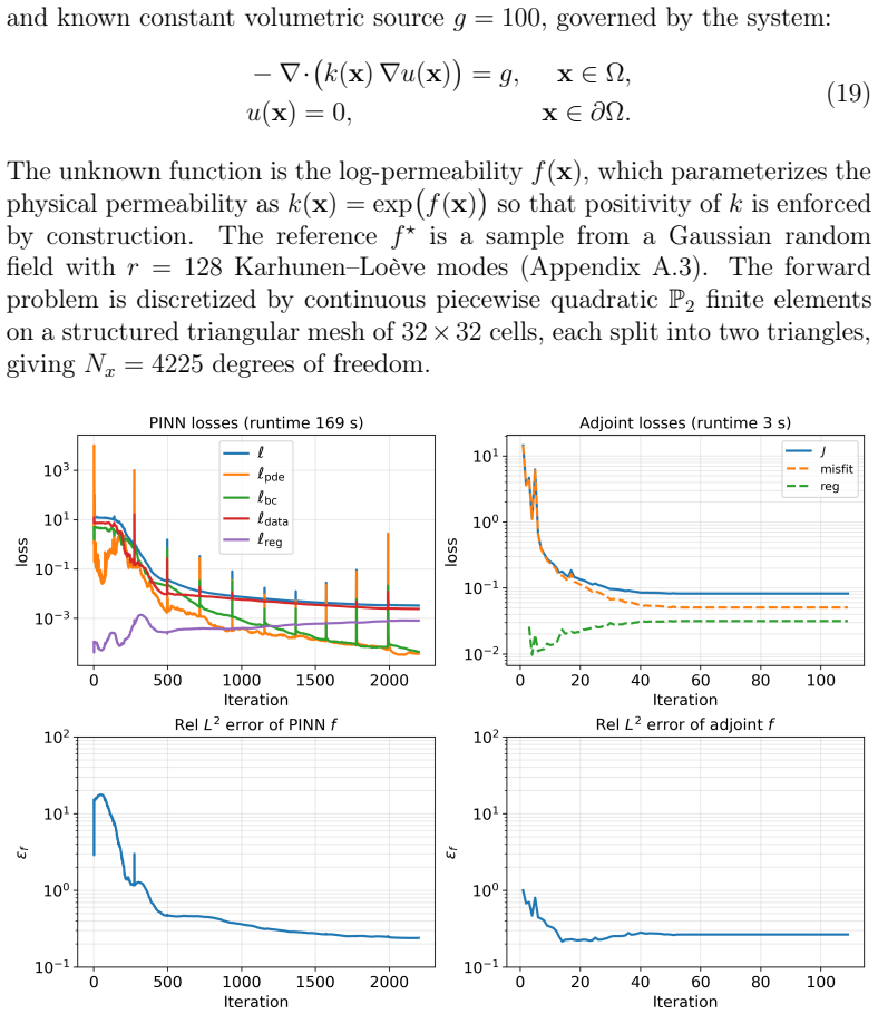
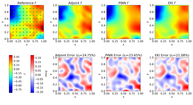
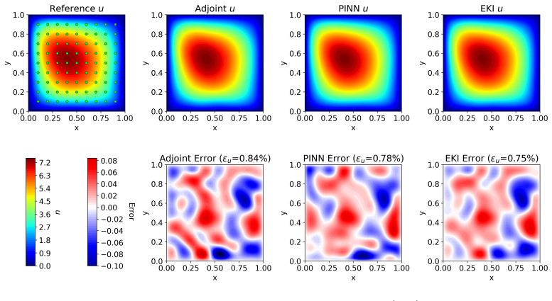
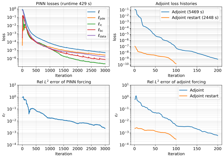
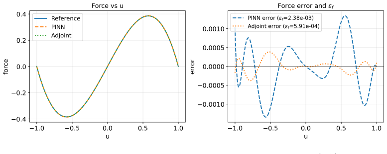
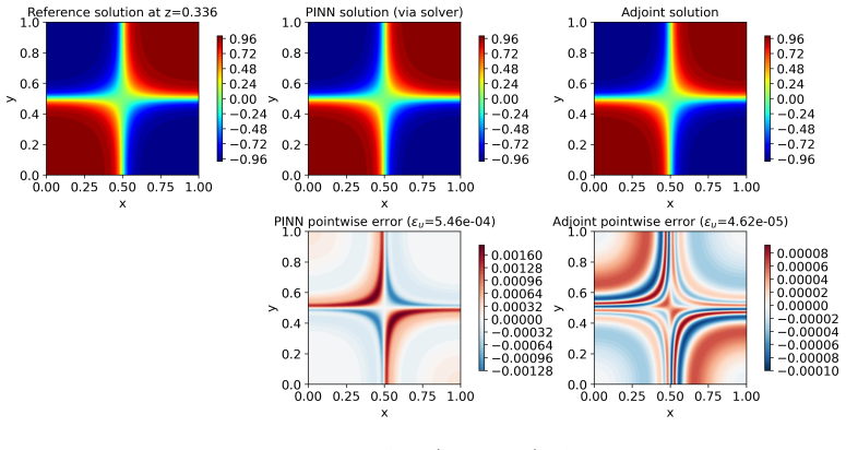
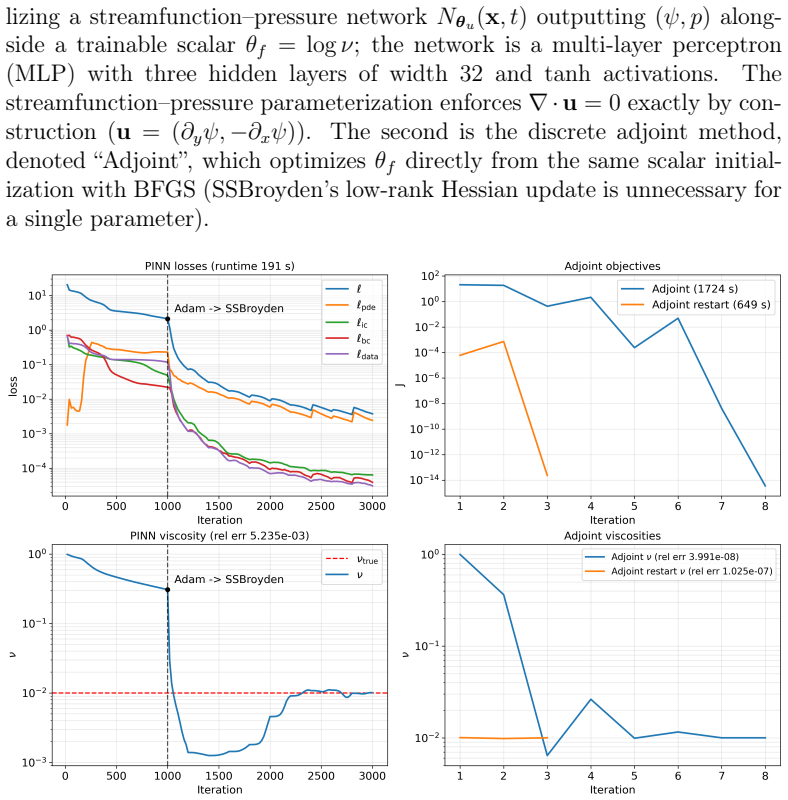
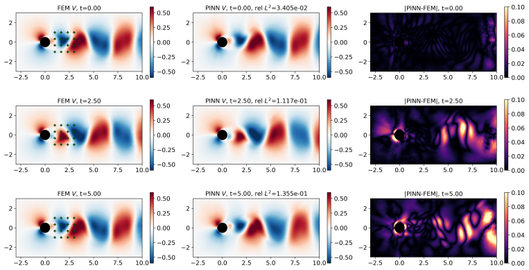
Inverse problems governed by partial differential equations (PDEs) are central to computational mechanics and are commonly solved by adjoint-based optimization, while physics-informed neural networks (PINNs) have emerged as a flexible alternative. Their relative performance remains difficult to assess because the two approaches are often compared under different formulations, parameterizations, optimizers, and regularization choices. We present a fair comparison of adjoint optimization and PINNs for PDE-constrained inverse problems. From a common abstract formulation, we instantiate both methods on identical domains, governing equations, observation models, and regularization terms, while matching the optimizer, unknown parameterization, and arithmetic precision wherever applicable. The benchmarks include unsteady Burgers, noisy Darcy permeability inversion, three-dimensional Allen--Cahn reaction identification, and unsteady Navier--Stokes viscosity identification. The results show that the representation of the unknown largely determines the preferred method: grid-based fields favor the discrete adjoint, whereas neural representations are native to PINNs and relevant for closure and constitutive modeling. For time-dependent problems, adjoint inversion can be dominated by trajectory storage and differentiation, while PINNs provide satisfactory reconstructions at lower cost. A PINN-warm-started adjoint strategy then recovers adjoint-level accuracy at substantially reduced cost.
Editorial analysis
A structured set of objections, weighed in public.
Referee Report
Summary. The paper claims to deliver a fair empirical comparison of discrete adjoint optimization versus PINNs for PDE-constrained inverse problems. Starting from a common abstract formulation, both methods are instantiated on identical domains, governing equations, observation models, and regularization terms, with optimizer, unknown parameterization, and arithmetic precision matched wherever applicable. Four benchmarks (unsteady Burgers, noisy Darcy, 3D Allen-Cahn, unsteady Navier-Stokes) are used to conclude that the representation of the unknown largely determines the preferred method: grid-based fields favor the discrete adjoint while neural representations are native to PINNs; adjoint methods suffer from trajectory storage costs in time-dependent cases, while a PINN-warm-started adjoint recovers accuracy at reduced cost.
Significance. If the comparisons are shown to be free of confounding mismatches, the work supplies concrete, benchmark-level guidance on method selection in computational mechanics and constitutive modeling. The multi-benchmark design and the hybrid warm-start strategy are positive features that could be useful to practitioners.
major comments (2)
- [Abstract] Abstract: the qualifier 'wherever applicable' for matching optimizer, parameterization, arithmetic precision, and gradient computation is load-bearing for the central claim that performance differences can be attributed to representation type alone. Without an explicit enumeration (in §2 or §3) of which cells of the comparison grid could not be matched and the quantitative effect of any residual differences, the attribution to representation remains unverified and the generalization beyond the four benchmarks is weakened.
- [Results] Results section (benchmarks): the claim that grid-based fields favor the discrete adjoint while neural representations favor PINNs requires explicit side-by-side runs in which the same representation is inverted by both methods (e.g., discrete adjoint applied to a neural parameterization of the unknown). If such cross-representation experiments are absent, the reported performance gaps cannot be cleanly separated from representation effects.
minor comments (2)
- [Methods] Clarify in the methods section how arithmetic precision and optimizer hyperparameters were enforced to be identical when one method uses automatic differentiation and the other uses discrete adjoints.
- [Figures] Figure captions should state the exact number of optimization iterations, wall-clock times, and error norms reported so that readers can reproduce the cost-accuracy trade-offs without re-deriving them from the text.
Simulated Author's Rebuttal
We thank the referee for the constructive comments, which help clarify the attribution of performance differences. We address each major comment below and commit to revisions that strengthen the manuscript without altering its core claims.
read point-by-point responses
-
Referee: [Abstract] Abstract: the qualifier 'wherever applicable' for matching optimizer, parameterization, arithmetic precision, and gradient computation is load-bearing for the central claim that performance differences can be attributed to representation type alone. Without an explicit enumeration (in §2 or §3) of which cells of the comparison grid could not be matched and the quantitative effect of any residual differences, the attribution to representation remains unverified and the generalization beyond the four benchmarks is weakened.
Authors: We agree that an explicit enumeration would make the 'wherever applicable' qualifier more transparent and support the central claim. In the revised manuscript we will add a dedicated subsection (or table) in §2 that lists, for each benchmark, every element of the comparison grid (optimizer, parameterization, arithmetic precision, gradient computation) together with whether it was matched and the quantitative effect of any residual mismatch. This directly addresses the concern about unverified attribution. revision: yes
-
Referee: [Results] Results section (benchmarks): the claim that grid-based fields favor the discrete adjoint while neural representations favor PINNs requires explicit side-by-side runs in which the same representation is inverted by both methods (e.g., discrete adjoint applied to a neural parameterization of the unknown). If such cross-representation experiments are absent, the reported performance gaps cannot be cleanly separated from representation effects.
Authors: The manuscript compares the two methods in their standard, computationally practical configurations (grid-based unknowns with the discrete adjoint; neural representations with PINNs), which is the setting most relevant to practitioners. Nevertheless, the referee correctly notes that cross-representation runs would further isolate representation effects from method effects. We will therefore add a short discussion subsection that (i) explains the technical obstacles to performing a full cross (e.g., memory and differentiability requirements when applying a discrete adjoint to a neural field) and (ii) reports any feasible preliminary cross-experiments or explicitly flags their absence as a limitation. This revision clarifies the scope of the attribution claim. revision: partial
Circularity Check
Empirical method comparison with no derivation chain
full rationale
This paper conducts an empirical benchmark comparison of adjoint optimization versus PINNs on four PDE inverse problems, matching conditions wherever applicable and reporting observed performance differences. No first-principles derivations, fitted predictions, or self-citation chains are present that reduce any central claim to its inputs by construction. The representation-based conclusion follows directly from the numerical results on external benchmarks rather than from any tautological redefinition or imported uniqueness theorem.
Axiom & Free-Parameter Ledger
Reference graph
Works this paper leans on
-
[1]
J. L. Lions, Optimal Control of Systems Governed by Partial Differential Equations, Springer-Verlag, 1971
1971
-
[2]
M. Hinze, R. Pinnau, M. Ulbrich, S. Ulbrich, Optimization with PDE Constraints, Vol. 23 of Mathematical Modelling: Theory and Applica- tions, Springer, Dordrecht, 2009.doi:10.1007/978-1-4020-8839-1
-
[3]
K. Duraisamy, G. Iaccarino, H. Xiao, Turbulence modeling in the age of data, Annual Review of Fluid Mechanics 51 (2019) 357–377.doi: 10.1146/annurev-fluid-010518-040547
-
[4]
G. E. Karniadakis, I. G. Kevrekidis, L. Lu, P. Perdikaris, S. Wang, L. Yang, Physics-informed machine learning, Nature Reviews Physics 3 (6) (2021) 422–440.doi:10.1038/s42254-021-00314-5. 27
-
[5]
A. Jameson, Aerodynamic design via control theory, Journal of Scientific Computing 3 (3) (1988) 233–260.doi:10.1007/BF01061285
-
[6]
M. B. Giles, N. A. Pierce, An introduction to the adjoint approach to design, Flow, Turbulence and Combustion 65 (3) (2000) 393–415
2000
-
[7]
C. S. Skene, M. F. Eggl, P. J. Schmid, A parallel-in-time approach for accelerating direct-adjoint studies, Journal of Computational Physics 429 (2021) 110033.doi:10.1016/j.jcp.2020.110033
-
[8]
R. D. Nzoyem, D. A. W. Barton, T. Deakin, A comparison of mesh- free differentiable programming and data-driven strategies for optimal control under PDE constraints, in: Proceedings of the SC ’23 Work- shops of the International Conference on High Performance Computing, Network, Storage, and Analysis (SC-W ’23), Association for Computing Machinery, 2023, ...
-
[9]
A. Alla, A. Pacifico, M. Palladino, A. Pesare, Online identification and control of pdes via reinforcement learning methods, Adv Comput Math 50 (2024)
2024
-
[10]
A. Alla, A. Pacifico, A pod approach to identify and control pdes on- line through state dependent riccati equations, Dyn Games Appl 15 (1) (2025) 481–502
2025
-
[11]
Raissi, P
M. Raissi, P. Perdikaris, G. E. Karniadakis, Physics-informed neural networks: A deep learning framework for solving forward and inverse problems involving nonlinear partial differential equations, Journal of Computational Physics 378 (2019) 686–707
2019
-
[12]
A. G. Baydin, B. A. Pearlmutter, A. A. Radul, J. M. Siskind, Auto- matic differentiation in machine learning: a survey, Journal of Machine Learning Research 18 (1) (2018) 5595–5637
2018
-
[13]
Kiyani, K
E. Kiyani, K. Shukla, J. F. Urbán, J. Darbon, G. E. Karniadakis, Optimizing the optimizer for physics-informed neural networks and kolmogorov-arnold networks, Computer Methods in Applied Mechan- ics and Engineering 446 (2025) 118308. 28
2025
-
[14]
A. Alla, G. Bertaglia, E. Calzola, A pinn approach for the online identi- fication and control of unknown pdes, Journal of Optimization Theory and Applications 206 (1) (2025) 8
2025
-
[15]
S. Mowlavi, S. Nabi, Optimal control of PDEs using physics-informed neural networks, Journal of Computational Physics 473 (2023) 111731. doi:10.1016/j.jcp.2022.111731
-
[16]
S. Gratton, A. Sartenaer, P. L. Toint, Recursive trust-region methods for multiscale nonlinear optimization, SIAM Journal on Optimization 19 (1) (2008) 414–444.doi:10.1137/050623012
-
[17]
C. Bunks, F. M. Saleck, S. Zaleski, G. Chavent, Multiscale seismic wave- form inversion, Geophysics 60 (5) (1995) 1457–1473.doi:10.1190/1. 1443880
work page doi:10.1190/1 1995
-
[18]
Z. Zhang, S. Liu, A. Alla, J. Darbon, G. E. Karniadakis, PINNs in PDE constrained optimal control problems: Direct vs indirect methods, arXiv preprint arXiv:2604.04920 (2026)
Pith/arXiv arXiv 2026
-
[19]
Glorot, Y
X. Glorot, Y. Bengio, Understanding the difficulty of training deep feed- forward neural networks, in: Proceedings of the thirteenth international conference on artificial intelligence and statistics, JMLR Workshop and Conference Proceedings, 2010, pp. 249–256
2010
-
[20]
M. A. Iglesias, K. J. Law, A. M. Stuart, Ensemble kalman methods for inverse problems, Inverse Problems 29 (4) (2013) 045001
2013
-
[21]
G. Strang, The discrete cosine transform, SIAM Review 41 (1) (1999) 135–147.doi:10.1137/S0036144598336745
-
[22]
M. Raissi, Z. Wang, M. S. Triantafyllou, G. E. Karniadakis, Deep learn- ing of vortex-induced vibrations, Journal of Fluid Mechanics 861 (2019) 119–137.doi:10.1017/jfm.2018.872
-
[23]
S. Cai, Z. Wang, S. Wang, P. Perdikaris, G. E. Karniadakis, Physics- informed neural networks for heat transfer problems, Journal of Heat Transfer 143 (6) (2021) 060801.doi:10.1115/1.4050542. 29 Appendix A. Implementation Details This appendix collects the discretization, parameterization, regulariza- tion, and optimization details deferred from Section 3...
discussion (0)
Sign in with ORCID, Apple, or X to comment. Anyone can read and Pith papers without signing in.