REVIEW 4 major objections 6 minor 60 references
Improved Approximations for Collective Neutrino Oscillations
T0 review · 4 major / 6 minor · reviewed 2026-08-05 · deepseek-v4-flash
Pith's one-line read Truncating the neutrino many-body hierarchy at second order reproduces Trotterized dynamics about two orders of magnitude better than mean field, at polynomial classical cost.
desk verdict Promising second-order cumulant closure, but the large-N physics claims outrun the validation. read the letter →
The pith
A machine-rendered reading of the paper's core claim, the machinery that carries it, and where it could break.
The reading
What carries the argument
The machinery is the BBGKY cumulant hierarchy on the product-structure basis of u(n^N): every operator is expanded in products of single-site su(n) generators Λ_Aμ, and the evolution of the one-body expectation value Φ_Aa and the two-body expectation value Γ_AaBb is closed by setting the third-order cumulant to zero. The resulting coupled ODEs (Eqs. 49 and 52) retain the antisymmetric part of Γ that drives entropy production, and the sparsity of the structure constants together with the (A,a)↔(B,b) symmetry of Γ gives polynomial scaling O(N^3 n^6).
What would settle it
Evolve a small system (say N≤8, n=2 or 3) exactly, compute the three-body cumulant ⟨δΛδΛδΛ⟩ along the trajectory, and compare its contribution in Eq. (52) with the one- and two-body terms; if it becomes comparable near μ(t)∼|B̄|, the closure—and with it the large-N phase-transition conclusions—fails.
Extended reading notes
Core claim
The central claim is that the BBGKY hierarchy for a one- and two-body su(n) Hamiltonian can be closed at second order—neglecting the fully connected three-body cumulant, ⟨δΛ_Aa δΛ_Bb δΛ_Cc⟩ = 0 in Eq. (52)—without losing the physics that mean field throws away. Equations (49) and (52) then form a closed, finite set of ordinary differential equations for the one-body expectation values Φ_Aa = ⟨Λ_Aa⟩ and the two-body expectation values Γ_AaBb = ⟨Λ_Aa Λ_Bb⟩. The truncation keeps the antisymmetric part of Γ, which is precisely the term that drives one-body entropy production and is identically zero at mean-field level. The paper validates this against a Trotterized evolution for N=4, n=3, findin
Load-bearing premise
The hierarchy is closed by assuming that three-neutrino connected correlations are exactly zero, and the paper offers no independent check that this stays true for the large systems where its main conclusions live.
Editorial extensions
If this is right
- At mean-field level the one-body entropy production is identically zero; the second-order closure removes that artifact, so entropy growth becomes accessible classically.
- The method reaches N=100 (two-flavor) and N=50 (three-flavor) with Monte Carlo angular averaging, sizes where exact evolution is impossible.
- The order parameter changes sharply near μ(t)∼|B̄| in both su(2) and su(3), supporting a dynamical phase transition in both cases.
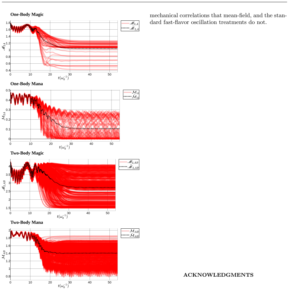
- Two-body magic and mana stay nonzero at late times, indicating the post-transition neutrino state is not stabilizer-simulable and remains non-trivial.
- Truncating at order m costs O((N choose m)(n^2−1)^m), so the scheme is systematically improvable toward the exponential exact limit.
Reading between the lines
- The paper's three-body entropy and mutual-information numbers are computed from one- and two-body data after the three-body cumulant has been set to zero, so the reported weak scrambling is a statement about what those lower-order operators carry, not a direct measurement of the neglected connected three-body correlation.
- Because the algebraic closure applies to any quadratic su(n) all-to-all Hamiltonian, the same O(N^3 n^6) scheme could be run on spin, Hubbard, or SYK-type models; the paper notes the common algebraic class but does not carry out those applications.
- A convergence test the paper does not perform—evolving a small N system exactly and monitoring the magnitude of the third-order cumulant—would map the regime where the large-N phase-transition and scrambling conclusions are safe.
- The angular averaging is done by Monte Carlo; increasing the number of angle samples or using low-discrepancy sampling would sharpen the reported momentum-space heat maps and test whether the delocalization pattern is converged.
Signed reviews
Editorial analysis
A structured set of objections, weighed in public.
Referee Report
Summary. The paper proposes a polynomial-scaling classical method for one- and two-body expectation values of quadratic su(n)-type many-body Hamiltonians, with collective neutrino oscillations as the target. The authors exploit the product structure of u(n^N), express the density matrix, entropy, Wigner functions, and magic in terms of operator moments, and close the BBGKY hierarchy at second order by setting the three-body cumulant to zero in Eq. (52). This yields coupled ODEs for the one-body and two-body expectation values with claimed O(N^3 n^6) cost. A single N=4, n=3, mu(0)=5 Trotter comparison (Figs. 2-4) shows roughly two orders of magnitude improvement over mean field for the moments and close agreement for entropy and magic. The large-N simulations (N=100 for su(2), N=50 for su(3)) are then used to claim a dynamical phase transition, momentum-space information delocalization, weak information scrambling, and persistent non-stabilizer magic.
Significance. If the method is valid at large N, it is a useful and general tool: it is independent of fitted parameters, has explicit polynomial cost, and the single Trotter benchmark is a genuine external check. The algebraic construction of entanglement and magic measures in the su(n) basis is also a useful contribution. However, the central physical claims depend on an unvalidated closure and on a projection step. The paper's contribution is therefore conditional: the formalism is promising, but the evidence presented does not yet establish the reliability of the second-order truncation in the crossover regime where the N=100 and N=50 conclusions are drawn.
major comments (4)
- [Sec. V.B; Sec. III.B] The only exact validation is a single N=4, n=3, mu(0)=5 Trotter run (Figs. 2-4), far from the large-N crossover. The suppression estimate in Eqs. (60)-(61) is O(mu^2/N^2); at N=100 and mu~5 this is ~2.5e-3 before O(1) prefactors, not negligible, and the estimate is perturbative in a strong-coupling regime. The paper does not report the size of the neglected third cumulant <delta-Lambda delta-Lambda delta-Lambda> during the N=100/N=50 runs. Please add exact small-system benchmarks over a range of N, n, mu(0), and crossing parameters; a time-step convergence study; and diagnostics measuring the neglected cumulant, or a comparison with a third-order truncation, to show that the closure is accurate where the physical conclusions are drawn.
- [Sec. IV.A, Eqs. (64)-(65)] At each step the algorithm projects Phi and Gamma back to the nearest bound when inequalities (64)-(65) fail. This clamping can hide positivity violations introduced by the truncation. The manuscript gives no statistics on how often or by how much the bounds are violated, and no demonstration that observables are insensitive to the projection. Since the phase-transition and scrambling claims are made in a regime where the closure is least tested, the projection could be shaping those results. Please report violation frequency and magnitude and, where possible, results without projection or with a less invasive regularization.
- [Sec. V.C, Figs. 6-17] The large-N results average over sampled Pi_AB ('100 independent' for su(2), 'fifty different Pi_ABs a hundred times' for su(3)), but no error bars or convergence in the number of angle samples are shown. The identification of a sharp crossover in the order parameter and the negativity of the three-body mutual information need uncertainty quantification; without it, one cannot distinguish physical transitions from Monte Carlo sampling noise. Please provide standard errors, sample-size convergence, and a criterion for the phase-transition time.
- [Sec. II.C.1, Eq. (20); Sec. V.C, Figs. 10 and 16] Computing the three-body entropy in Eq. (20) requires three-body expectation values, but the evolution only tracks one- and two-body moments. Any S_3 used in the mutual-information estimator must be reconstructed by setting the third cumulant to zero in Eq. (47d). Thus the negative three-body mutual information is not an independent signature of scrambling; it is largely a restatement of the closure. Please state this reconstruction explicitly and validate it against exact small-N data or a higher-order closure before claiming weak information scrambling.
minor comments (6)
- [Sec. II.C.1] Typo: 'weather' should be 'whether'. Also, the 'naive mutual information' is acknowledged not to be the formal Renyi mutual information; this caveat should be repeated whenever the estimator is used to claim scrambling.
- [Sec. III.B, Eq. (52)] The notation \bar{g} and the index contractions in Eq. (52) are not defined in the text. The terms involving Pi_AB, Pi_AC, and the xi factors need a clearer derivation or a supporting appendix.
- [Sec. IV.A, Eq. (66)] The expression lim_{delta t -> 0} ... is not an update rule as written. Please specify how the Lagrange-multiplier constraint is applied at finite time steps and how the limit is implemented in the RK4 scheme.
- [Fig. 1] The scaling plot reports only fitted curves from OLS. Please give the fitted beta_i values and run-to-run variability, and compare against actual Trotter runtimes for the same N, since 'sub-exponential' is a central complexity claim.
- [Sec. V] Please provide a table of initial conditions, mixing parameters, and all simulation parameters. Currently 'all electron neutrinos' and the mixing angles appear in text only, which makes reproducibility harder.
- [General] No data or code availability statement is included. For a numerical paper of this type, releasing the ODE solver and Trotter comparison code would strengthen reproducibility.
Circularity Check
No significant circularity: the central claim is benchmarked against an independent Trotter simulation, and no fitted parameters are disguised as predictions.
full rationale
The paper's central numerical claim is that second-order BBGKY truncation, obtained by setting the three-body cumulant to zero in Eq. (52), tracks the exact Trotter evolution of the one- and two-body operators about two orders of magnitude better than mean field. This is not circular: the Trotter result is an independent solution of the same Hamiltonian Eq. (41) for N=4, n=3, μ(0)=5, and the comparison quantities ΔΦ² and ΔΓ² are direct error metrics rather than parameters fitted to the benchmark. The closure assumption itself is an uncontrolled approximation, and the lack of large-N exact checks is a legitimate correctness/validation concern, but it is not a circularity because the closure is not derived from, or fitted to, the quantities it is used to predict. The authors do cite their own prior work, notably Refs. [6] and [40], for the algebraic product-structure framework and the stationary-phase connection to mean-field theory, but these citations provide background formalism and are not the load-bearing evidence for the new truncation result; the relevant equations are rederived in Sections II and III. No uniqueness theorem, no ansatz smuggled through self-citation, and no renaming of a known result forces the conclusions. The low score reflects only the presence of self-citations that are not load-bearing.
Assumptions & free parameters
free parameters (2)
- Initial neutrino-neutrino coupling mu(0) =
5 (dimensionless, mu0 in Eq. (67))
- Bulb-model radius r0 =
not specified; chosen such that mu-bar(0) is proportional to omega0
assumptions (5)
- domain assumption The forward-scattering collective neutrino oscillation Hamiltonian is of the form Eq. (41) with one- and two-body su(n) interactions.
- standard math The Gell-Mann basis and structure constants f, d, g obey Eqs. (1)-(4) and Eq. (12).
- ad hoc to paper The third-order cumulant <delta-Lambda_Aa delta-Lambda_Bb delta-Lambda_Cc> is set to zero to close the hierarchy.
- domain assumption Angular degrees of freedom can be integrated by uniform Monte Carlo sampling over the 2-sphere using Eq. (68).
- domain assumption Trotterized evolution with adaptive time step is an accurate benchmark for N=4, n=3.
Cite this review
Pith. "Pith review of Improved Approximations for Collective Neutrino Oscillations." pith.science (2026). https://pith.science/paper/5ZLQGK6W
@misc{pith2026260728619,
  author       = {Pith},
  title        = {Pith review of: Improved Approximations for Collective Neutrino Oscillations},
  year         = {2026},
  howpublished = {\url{https://pith.science/paper/5ZLQGK6W}},
  note         = {Machine review of arXiv:2607.28619}
}
abstract
A one- and two-body $\mathfrak{su}(n)$ Hamiltonian governing the dynamics of many systems, including collective neutrino oscillations, is investigated. We start by analyzing the algebraic structure($\mathfrak{u}(n^N)$), formulate a product structure of the algebra, and utilize this to construct generic expressions for operator expectation values, R\'{e}nyi Entropy, and Wigner Functions. Performing BBGKY hierarchy truncation we develop a systematic methodology for going beyond the mean field with polynomial scaling on a classical computer.
Figures


Figures from the paper (9 more)


Reference graph
Works this paper leans on
-
[1]
Operator Decomposition, Completeness, Operator Transformations, and Operator Action Since all possible products of Λ AµA ’s are Hermi- tian matrices of the fundamental representation of theu(n N ) algebra (for an explicit illustration see Ref. [40]) we can decompose any arbitraryn N ×n N matrix in terms of them: O= 1 nN Tr(O) + 1 nN−1 2 Tr OΛAa ΛAa +... =...
-
[2]
R´ enyi Entropy & R´ enyi Mutual Information In many-body physics, the entanglement structure is often the primary lens through which we exam- ine the behavior of largeN-systems. To examine the entanglement structure, we introduce the R´ enyi En- tropy: Sα,{A} = 1 1−α ln Tr ρα {A} (19) Forα= 1 R´ enyi Entropy reduces to the von Neumann entropy. Forα= 2, U...
-
[3]
Discrete Phase Space and Mana Another fundamental characteristic of these many- body systems is their representation in phase space via the Wigner function. The Wigner function provides a quasi probability distribution that maps the many- body density matrix onto a discrete phase space, of- fering a direct visual and mathematical diagnostic of quantum non...
-
[4]
Mana to Magic The Gottesman-Knill theorem states that quantum systems that utilize only stabilizer resources, i.e. cir- cuits that only consist of gates from the Pauli or Clif- ford groups, can be efficiently simulated in polynomial time on a probabilistic classical computer [45]. Thus, it is important to have a measure for the amount of non-stabilizer re...
-
[5]
H. Duan, G. M. Fuller, and Y.-Z. Qian, Ann. Rev. Nucl. Part. Sci.60, 569 (2010), arXiv:1001.2799 [hep- ph]
arXiv 2010
-
[6]
A. B. Balantekin, J. Phys. G45, 113001 (2018), arXiv:1809.02539 [hep-ph]
work page Pith review arXiv 2018
-
[7]
I. Tamborra and S. Shalgar, Ann. Rev. Nucl. Part. Sci.71, 165 (2021), arXiv:2011.01948 [astro-ph.HE]
arXiv 2021
- [8]
Show all 60 references
-
[9]
M. C. Volpe, Rev. Mod. Phys.96, 025004 (2024), arXiv:2301.11814 [hep-ph]
2024 arXiv
-
[10]
A. B. Balantekin and Y. Pehlivan, J. Phys. G34, 47 (2007), arXiv:astro-ph/0607527
2007 arXiv
-
[11]
M. J. Cervia, A. V. Patwardhan, A. B. Balantekin, ‡. S. N. Coppersmith, and C. W. Johnson, Phys. Rev. D100, 083001 (2019), arXiv:1908.03511 [hep-ph]
2019 arXiv
-
[12]
M. J. Cervia, P. Siwach, A. V. Patwardhan, A. B. Balantekin, S. N. Coppersmith, and C. W. Johnson, Phys. Rev. D105, 123025 (2022), arXiv:2202.01865 [hep-ph]
2022 arXiv
-
[13]
Lacroix, A
D. Lacroix, A. B. Balantekin, M. J. Cervia, A. V. Pat- wardhan, and P. Siwach, Phys. Rev. D106, 123006 (2022), arXiv:2205.09384 [nucl-th]. 16
2022 arXiv
-
[14]
Illa and M
M. Illa and M. J. Savage, Phys. Rev. Lett.130, 221003 (2023), arXiv:2210.08656 [nucl-th]
2023 arXiv
-
[15]
J. D. Martin, A. Roggero, H. Duan, J. Carlson, and V. Cirigliano, Phys. Rev. D105, 083020 (2022), arXiv:2112.12686 [hep-ph]
2022 arXiv
-
[16]
J. D. Martin, D. Neill, A. Roggero, H. Duan, and J. Carlson, Phys. Rev. D108, 123010 (2023), arXiv:2307.16793 [hep-ph]
2023 arXiv
-
[17]
Carlson, A
J. Carlson, A. Roggero, and D. Neill, (2026), arXiv:2603.12192 [hep-ph]
2026
-
[18]
Lacroix, A
D. Lacroix, A. Bauge, B. Yilmaz, M. Mangin-Brinet, A. Roggero, and A. B. Balantekin, Phys. Rev. D110, 103027 (2024), arXiv:2409.20215 [hep-ph]
2024 arXiv
-
[19]
Neill, H
D. Neill, H. Liu, J. Martin, and A. Roggero, Phys. Rev. Res.7, 023157 (2025), arXiv:2406.18677 [hep- ph]
2025 arXiv
-
[20]
Chernyshev, C
I. Chernyshev, C. E. P. Robin, and M. J. Savage, Phys. Rev. Res.7, 023228 (2025), arXiv:2411.04203 [quant-ph]
2025 arXiv
-
[21]
Bhaskar, A
R. Bhaskar, A. Roggero, and M. J. Savage, Phys. Rev. C110, 045801 (2024)
2024
-
[22]
Br¨ okemeier, S
F. Br¨ okemeier, S. M. Hengstenberg, J. W. T. Keeble, C. E. P. Robin, F. Rocco, and M. J. Savage, Phys. Rev. C111, 034317 (2025), arXiv:2409.12064 [nucl- th]
2025 arXiv
-
[23]
O. Kiss, I. Tavernelli, F. Tacchino, D. Lacroix, and A. Roggero, (2025), arXiv:2510.24841 [quant-ph]
2025
-
[24]
Laraib and S
Z. Laraib and S. Richers, Phys. Rev. D112, L101304 (2025), arXiv:2507.02040 [astro-ph.HE]
2025 arXiv
-
[25]
Laraib and S
Z. Laraib and S. Richers, Phys. Rev. D112, 123045 (2025), arXiv:2511.16506 [astro-ph.HE]
2025 arXiv
- [26]
-
[27]
Froustey, E
J. Froustey, E. Rrapaj, Y. Liu, G. Li, C. Iancu, and V. Cirigliano, (2026), arXiv:2606.12404 [hep-ph]
2026 arXiv
-
[28]
Yeter-Aydeniz, S
K. Yeter-Aydeniz, S. Bangar, G. Siopsis, and R. C. Pooser, Quant. Inf. Proc.21, 84 (2022), arXiv:2104.03273 [quant-ph]
2022 arXiv
-
[29]
Amitrano, A
V. Amitrano, A. Roggero, P. Luchi, F. Turro, L. Vespucci, and F. Pederiva, Phys. Rev. D107, 023007 (2023), arXiv:2207.03189 [quant-ph]
2023 arXiv
-
[30]
B. Hall, A. Roggero, A. Baroni, and J. Carlson, Phys. Rev. D104, 063009 (2021), arXiv:2102.12556 [quant- ph]
2021 arXiv
-
[31]
Siwach, K
P. Siwach, K. Harrison, and A. B. Balantekin, Phys. Rev. D108, 083039 (2023), arXiv:2308.09123 [quant- ph]
2023 arXiv
-
[32]
A. B. Balantekin, M. J. Cervia, A. V. Patwardhan, E. Rrapaj, and P. Siwach, Eur. Phys. J. A59, 186 (2023), arXiv:2305.01150 [nucl-th]
2023 arXiv
-
[33]
Turro, I
F. Turro, I. A. Chernyshev, R. Bhaskar, and M. Illa, Phys. Rev. D111, 043038 (2025), arXiv:2407.13914 [quant-ph]
2025 arXiv
-
[34]
Spagnoliet al., Phys
L. Spagnoliet al., Phys. Rev. D111, 103054 (2025), arXiv:2503.00607 [quant-ph]
2025 arXiv
-
[35]
D. J. Heimsoth, A. B. Balantekin, and P. Siwach, Three-flavor supernova neutrino simulation using a hybrid quantum-classical algorithm with qutrits (2026), arXiv:2605.01099 [hep-ph]
2026 arXiv
- [36]
-
[37]
Mangin-Brinet, A
M. Mangin-Brinet, A. Bauge, and D. Lacroix, Phys. Rev. D113, 036026 (2026), arXiv:2507.18482 [hep- ph]
2026 arXiv
-
[38]
Volpe, D
C. Volpe, D. V¨ a¨ an¨ anen, and C. Espinoza, Phys. Rev. D87, 113010 (2013), arXiv:1302.2374 [hep-ph]
2013 arXiv
-
[39]
V¨ a¨ an¨ anen and C
D. V¨ a¨ an¨ anen and C. Volpe, Phys. Rev. D88, 065003 (2013), arXiv:1306.6372 [hep-ph]
2013 arXiv
-
[40]
Serreau and C
J. Serreau and C. Volpe, Phys. Rev. D90, 125040 (2014), arXiv:1409.3591 [hep-ph]
2014 arXiv
-
[41]
Bossion and P
D. Bossion and P. Huo, General formulas of the structure constants in thesu(n) lie algebra (2021), arXiv:2108.07219 [math-ph]
2021 arXiv
- [42]
-
[43]
Kitaev, Annals Phys.321, 2 (2006), arXiv:cond- mat/0506438
A. Kitaev, Annals Phys.321, 2 (2006), arXiv:cond- mat/0506438
2006
-
[44]
A. B. Balantekin and A. M. Suliga, Eur. Phys. J. A 60, 124 (2024), arXiv:2405.13862 [quant-ph]
2024 arXiv
-
[45]
´A. M. Alhambra, PRX Quantum4, 040201 (2023), arXiv:2204.08349 [quant-ph]
2023 arXiv
-
[46]
S. O. Scalet, ´A. M. Alhambra, G. Styliaris, and J. I. Cirac, Quantum5, 541 (2021), arXiv:2103.01709 [quant-ph]
2021 arXiv
-
[47]
Seshadri, V
A. Seshadri, V. Madhok, and A. Lakshminarayan, Phys. Rev. E98, 052205 (2018), arXiv:1806.00113 [quant-ph]
2018 arXiv
-
[48]
G. Bjrk, A. B. Klimov, and L. L. Snchez-Soto (Else- vier, 2008) pp. 469–516
2008
-
[49]
Gottesman, in22nd International Colloquium on Group Theoretical Methods in Physics(1998) pp
D. Gottesman, in22nd International Colloquium on Group Theoretical Methods in Physics(1998) pp. 32– 43, arXiv:quant-ph/9807006
1998 arXiv
-
[50]
Leone, S
L. Leone, S. F. E. Oliviero, and A. Hamma, Phys. Rev. Lett.128, 050402 (2022), arXiv:2106.12587 [quant-ph]
2022 arXiv
-
[51]
Salasnich and C
L. Salasnich and C. Vianello, SciPost Phys. Lect. Notes117, 1 (2026)
2026
-
[52]
R. Kubo, J. Phys. Soc. Jap.17, 1100 (1962)
1962
-
[53]
M. E. Peskin and D. V. Schroeder,An Introduction to quantum field theory(Addison-Wesley, Reading, USA, 1995)
1995
-
[54]
Cirigliano, S
V. Cirigliano, S. Sen, and Y. Yamauchi, Phys. Rev. D 110, 123028 (2024), arXiv:2404.16690 [hep-ph]
2024 arXiv
-
[55]
M. J. Cervia, Phys. Rev. D113, 043010 (2026), arXiv:2510.22005 [hep-ph]
2026
-
[56]
Kuehn, Moment closure—a brief review, inCon- trol of Self-Organizing Nonlinear Systems, edited by E
C. Kuehn, Moment closure—a brief review, inCon- trol of Self-Organizing Nonlinear Systems, edited by E. Sch¨ oll, S. H. L. Klapp, and P. H¨ ovel (Springer In- ternational Publishing, Cham, 2016) pp. 253–271
2016
-
[57]
H. Duan, G. M. Fuller, J. Carlson, and Y.-Z. Qian, Phys. Rev. D74, 105014 (2006), arXiv:astro- ph/0606616
2006
-
[58]
Hilfer, B
R. Hilfer, B. Biswal, H.-G. Mattutis, and W. Janke, Computer Physics Communications169, 230 (2005), proceedings of the Europhysics Conference on Com- putational Physics 2004
2005
-
[59]
J. J. Wallman and S. D. Bartlett, Phys. Rev. A85, 062121 (2012), arXiv:1203.2652 [quant-ph]
2012 arXiv
-
[60]
R. J. Garcia, K. Bu, and A. Jaffe, Proc. Nat. Acad. Sci.120, e2217031120 (2023), arXiv:2208.10477 [quant-ph]. 17
2023 arXiv
Reviewed August 5, 2026 · model on record in the stance chip above.
Discussion (0). Continue with ORCID to comment.