REVIEW 4 major objections 5 minor 42 references
midr: Learning from Black-Box Models by Maximum Interpretation Decomposition
T0 review · 4 major / 5 minor · reviewed 2026-08-07 · deepseek-v4-flash
Pith's one-line read The midr package builds the most accurate low-order additive surrogate of any black-box prediction function, with strict centering so every effect can be read as a contribution.
desk verdict midr is a workmanlike package for a reasonable idea, but the fitted object may not satisfy the strict centering that powers the paper's headline claims. read the letter →
The pith
A machine-rendered reading of the paper's core claim, the machinery that carries it, and where it could break.
The reading
What carries the argument
The machinery has three parts. The first is the functional decomposition itself: effects $f_J$ indexed by feature subsets $J$, with order $|J|$, whose sum up to order $m$ defines the surrogate $F_m$. The second is the optimization that defines MID: minimize the uninterpreted variation ratio $U(F_m)$ subject to strict centering, $\mathbb{E}[f_J(X_J)\mid X_{J'}]=0$ for all proper $J'\subset J$, and zero higher-order effects, with uniqueness restored by minimizing the expected squared norm among all minimizers. The third is the computational engine: each effect is expanded in a piecewise constant or piecewise linear encoding basis with $k_j$ knots per feature, centering is imposed as linear constraints on a discrete grid for continuous features, and the whole problem becomes a constrained least squares problem solved with a choice of fast linear algebra methods. This same machinery yields a closed-form expression for Shapley values of the surrogate, so local attribution is a byproduct rather than a separate expensive computation.
What would settle it
On a synthetic model with correlated continuous features and a known closed-form MID, run midr at increasing grid resolutions; if the fitted surrogate's uninterpreted variation ratio does not converge to the theoretical optimum, or if some other strictly centered additive order-2 fit attains lower squared error on a large held-out sample, the implementation does not realize the paper's central claim.
Extended reading notes
Core claim
Maximum Interpretation Decomposition is a functional decomposition: the fitted prediction function $f$ is approximated by $\sum_{|J|\le m} f_J(x_J)$, an intercept plus main effects and interaction effects up to order $m$. The defining claim is that among all additive representations built from terms of order at most $m$ that also satisfy strict centering, meaning $\mathbb{E}[f_J(X_J)\mid X_{J'}]=0$ for every proper subset $J'\subset J$, the MID model of order $m$ minimizes the expected squared error, measured by the uninterpreted variation ratio $U(F_m)=\mathbb{E}[(f(X)-F_m(X))^2]/\mathrm{Var}(f(X))$. Strict centering is what makes each effect readable as a standalone contribution, and the same structure yields a closed-form Shapley attribution, $\phi^{ms}_{ij}=\sum_{J\ni j, |J|\le m}\frac{1}{|J|}f^{\mathrm{mid}}_J(x_{iJ})$. The package realizes this by encoding each feature in piecewise constant or piecewise linear basis functions, imposing centering as linear constraints on a discrete grid for continuous features, and solving a constrained least squares problem, with a minimum-norm rule restoring uniqueness when the solution is not unique. A regression-benchmark demonstration shows a near-zero uninterpreted variation ratio, and a correlated-features experiment shows MID main-effect plots tracking the true function instead of following the extrapolation artifacts that affect partial dependence plots.
Load-bearing premise
The central claim depends on the estimated, grid-discretized version of the decomposition being a faithful stand-in for the mathematically defined optimum, even when features are continuous and correlated.
Editorial extensions
If this is right
- Any black-box model can be summarized by main-effect and interaction plots that are, by construction, the best low-order additive approximation in squared error.
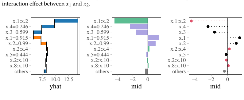
- The same surrogate supports local explanations: per-observation prediction breakdowns, conditional curves, and SHAP values computed exactly in closed form rather than by sampling.
- For correlated features, MID avoids the extrapolation distortion that affects partial dependence plots, because centering is imposed on observed conditional structure rather than on marginal averages.
- Users can check surrogate quality by the uninterpreted variation ratio on held-out predictions, so the method carries its own accuracy diagnostic.
- The package's computation cost is dominated by the constrained least squares solve and grows with the number of parameters, with faster solvers reducing runtime substantially.
Reading between the lines
- An implication the paper leaves implicit: the optimality claim is about the population problem, and the empirical solution depends on the chosen encoding basis and grid; finer grids should converge to the population MID, but the paper does not quantify that convergence.
- Another extension: the same formulation could be pushed to higher-order interactions or made sparse, selecting only the feature pairs that most reduce the uninterpreted variation ratio, which would help when many interactions are negligible.
- The 'most accurate' claim means among additive representations of the same order; if the black box is strongly non-additive, even the best order-2 MID will miss structure, so the package's diagnostic ratio, not the decomposition alone, should decide whether the surrogate is trustworthy.
- Because the closed-form Shapley values are Shapley values of the surrogate rather than of the original black box, their faithfulness to the original prediction is bounded by the surrogate's accuracy. This point deserves to be stated explicitly.
Editorial analysis
A structured set of objections, weighed in public.
Referee Report
Summary. The paper presents the R package midr, which implements Maximum Interpretation Decomposition (MID), a functional-decomposition method that approximates a black-box prediction function f by a low-order additive function minimizing expected squared error subject to strict centering of all effects. The manuscript reviews related work on PDP, ALE, SHAP, and ICE; defines MID and its numerical estimation by constrained least squares with piecewise-constant or piecewise-linear basis functions; and demonstrates the package on a Friedman regression benchmark, including main-effect and interaction plots, importance measures, ICE/breakdown/SHAP visualizations, a pragmatic-stability simulation with correlated features, and runtime comparisons for least-squares solvers.
Significance. If the theoretical and numerical claims hold, MID is an attractive global surrogate: it combines least-squares optimality with exactly centered components, which yields a closed-form SHAP decomposition (44) and a unified local-global interpretation. The paper's strengths are its clear connection to existing IML methods, a complete and reproducible R implementation with extensive code examples, and a useful numerical comparison of linear algebra backends. The central limitation is that the package solves a finite-dimensional grid-based version of the problem, and the manuscript does not supply the approximation theory needed to transfer the attractive population-level properties to the fitted object.
major comments (4)
- [Section 3, Definition, Eqs. (30)-(31)] Existence and uniqueness of the MID minimizer are asserted without proof: the text states that the decomposition is 'guaranteed to exist' and that uniqueness is obtained by selecting the minimum-norm solution among candidates, but the only reference is Iwasawa and Matsumori (2025), which is listed as 'Forthcoming'. Because the paper's headline optimality claim and the solver's tie-breaking procedure both depend on these properties, this is a load-bearing point. Please include a proof or a precise statement of the conditions under which existence and uniqueness hold, or clearly state them as assumptions imported from the forthcoming paper.
- [Section 3, Numerical estimation; Appendix, Eq. (63)] The empirical strict centering constraint (34) is not equivalent to the population constraint for continuous features. The appendix replaces E[f_pq(X_p,X_q)|X_p=x_p]=0 by the bin-level constraints sum_i chi^a_p(x_ip) f_pq(x_ip,x_iq)=0 for a=1,...,k_p, and symmetrically for q. These constraints are necessary but not sufficient for the population conditional expectation to vanish: a fitted interaction can satisfy every bin constraint while E[f_pq|X_p=x_p] is nonzero within a bin. The manuscript gives no grid-placement rule, no consistency theorem, and no approximation-error bound. Consequently, the object returned by interpret() is not shown to be the most accurate order-m additive representation, and the attribution property (41), used for breakdown plots and SHAP values, need not hold exactly for the fitted object. This gap should be addressed by a theorem connecting the grid solution to the population MID as n and k_j grow, or by clearly labeling the output as an approximate MID with appropriate diagnostics.
- [Section 3, Visualization; Section 6] The closed-form MID-Shapley values and the 'most accurate' claim are valid for the population MID defined by Eq. (30) with exact strict centering. The package, however, solves the finite-dimensional problem (65), whose feasible set differs from the MID class, as explained in the previous comment. The sentence in Section 6 that 'the MID model of order m is the most accurate global additive representation' should therefore be restricted to the population quantity, and the finite-basis solution should be presented as an approximation whose error is not yet quantified. In the same vein, the characteristic function in Eq. (43) drops all J not contained in S only because of strict centering; this equality may fail for the bin-level solution, so the 'exact' MID-derived SHAP values require either a proof of exact centering or a revision to describe them as approximations.
- [Appendix, Eqs. (57)-(59)] The tie-breaking criterion used in the solver is the weighted coefficient norm ||Delta^{1/2} beta||^2, where Delta is a diagonal matrix with entries sum_i chi^s_j(x_ij). This does not coincide with the criterion stated in Eq. (35), which minimizes sum_J sum_i f_J(x_iJ)^2. The two agree for the piecewise-constant encoding (50)-(51), where the basis functions have disjoint supports, but not for the piecewise-linear encoding (52), where X^T X has nonzero off-diagonal entries. Please clarify whether the weighted coefficient norm is an intentional solver choice; if so, it should be disclosed as a modification of Eq. (35), and if not, the solver should minimize the empirical norm actually specified there.
minor comments (5)
- [Section 4 and Abstract] The abstract and Section 4 mention classification models, but all demonstrations in the paper are regression examples; either add a small classification example or make the wording explicitly refer users to the vignettes for classification.
- [Figure 9 caption] The caption contains the typo 'newral network models'; it should read 'neural network models'.
- [Reference list] The bibliography entry for the package lists 'R. Asasihba', but the author name in the paper is 'Ryoichi Asashiba'; the spelling should be corrected.
- [Appendix, Eq. (52)] The boundary encoding functions are defined using ratios such as (x_j - x_j^(0))/(x_j^(1) - x_j^(0)) with x_j^(0) = -infinity, and the text says the ratio is taken to be 1; this should be phrased as a limit rather than an ordinary ratio.
- [Table 1] The runtime benchmark reports average evaluation times but does not state the number of replicates or provide standard errors; adding this information would make the comparison fully reproducible.
Circularity Check
Minor structural self-citation for MID's existence guarantee; no derivation reduces to a fitted value.
-
self citation load bearing
[Section 3, Definition (Eqs. 30-31); cf. Section 1 and bibliography entry 'Iwasawa and Matsumori, 2025, Forthcoming'.]
"The Maximum Interpretation Decomposition of order m is guaranteed to exist but is not necessarily unique."
The paper's target object, F_mid(m), is defined as the argmin in Eq. (30), and the well-posedness of that definition (existence, and uniqueness via Eq. (31)) is asserted without proof in this paper. The assertion rests on Iwasawa and Matsumori (2025), a forthcoming paper by one of the present authors, cited in Section 1 and Section 3. No independent proof, machine-checked certificate, or stated assumptions are provided, so the central premise that the package actually computes a well-defined MID relies on a same-author citation rather than on the paper's own derivation. This is a structural self-citation, though it is not used to fit any numerical output.
full rationale
The central numerical method is a constrained least-squares projection: the paper defines MID as the minimizer of the uninterpreted variation ratio in Eq. (30) and then solves the finite-basis problem in Eq. (65). The headline 'most accurate' claim in Section 6 is explicitly labeled 'By definition,' so it is a true definitional property rather than a hidden prediction; it does not reduce a fitted quantity to a renamed output. The simulations use a known Friedman function and standard benchmark data, so no fitted input is called a prediction in a load-bearing way. The main circularity burden is the existence/uniqueness guarantee for population MID, which is imported from the authors' own forthcoming paper without proof; this is a genuine self-citation, but it does not force any numerical result in the package. The gap between the population strict centering constraint and the discrete-grid empirical constraints in the Appendix is an approximation-error concern (correctness risk), not a circularity. Overall score 2: one minor structural self-citation, central derivation otherwise self-contained.
Assumptions & free parameters
free parameters (2)
- k_j (number of encoding functions per feature) =
k = c(25, 5) in examples; default package setting not stated
- kappa (penalty factor for centering constraints, alternative solver) =
not specified, only said to be >1
assumptions (3)
- ad hoc to paper Existence and uniqueness of MID under the stated conditions
- domain assumption Strict centering via conditional expectations is the right identifiability constraint for interpretability
- domain assumption Prediction function f is square-integrable and can be approximated by the chosen finite basis within the support of the feature distribution
Cite this review
Pith. "Pith review of midr: Learning from Black-Box Models by Maximum Interpretation Decomposition." pith.science (2026). https://pith.science/paper/624EJRTB
@misc{pith2026250608338,
  author       = {Pith},
  title        = {Pith review of: midr: Learning from Black-Box Models by Maximum Interpretation Decomposition},
  year         = {2026},
  howpublished = {\url{https://pith.science/paper/624EJRTB}},
  note         = {Machine review of arXiv:2506.08338}
}
read the original abstract
The use of appropriate methods of Interpretable Machine Learning (IML) and eXplainable Artificial Intelligence (XAI) is essential for adopting black-box predictive models in fields where model and prediction explainability is required. As a novel tool for interpreting black-box models, we introduce the R package midr, which implements Maximum Interpretation Decomposition (MID). MID is a functional decomposition approach that derives a low-order additive representation of a black-box model by minimizing the squared error between the model's prediction function and this additive representation. midr enables learning from black-box models by constructing a global surrogate model with advanced analytical capabilities. After reviewing related work and the theoretical foundation of MID, we demonstrate the package's usage and discuss some of its key features.
Figures


Figures from the paper (7 more)




Reference graph
Works this paper leans on
-
[1]
K. Aas, M. Jullum, and A. Løland. Explaining individual predictions when features are dependent: More accurate approximations to Shapley values. Artificial Intelligence, 298: 0 103502, 2021. ISSN 0004-3702. doi:https://doi.org/10.1016/j.artint.2021.103502. URL https://www.sciencedirect.com/science/article/pii/S0004370221000539
arXiv 2021
-
[2]
D. W. Apley and J. Zhu. Visualizing the effects of predictor variables in black box supervised learning models. Journal of the Royal Statistical Society Series B: Statistical Methodology, 82 0 (4): 0 1059--1086, 06 2020. ISSN 1369-7412. doi:10.1111/rssb.12377. URL https://doi.org/10.1111/rssb.12377
-
[3]
R. Asasihba and H. Iwasawa. midr: Learning from Black-Box Models by Maximum Interpretation Decomposition, 2025. URL https://github.com/ryo-asashi/midr. R package version 0.5.0, https://ryo-asashi.github.io/midr/
work page 2025
-
[4]
D. Bates and D. Eddelbuettel. Fast and elegant numerical linear algebra using the RcppEigen package. Journal of Statistical Software, 52 0 (5): 0 1--24, 2013. doi:10.18637/jss.v052.i05
-
[5]
P. Biecek. DALEX : Explainers for complex predictive models in R . Journal of Machine Learning Research, 19 0 (84): 0 1--5, 2018. URL https://jmlr.org/papers/v19/18-416.html
work page 2018
-
[6]
P. Biecek and T. Burzykowski. Explanatory Model Analysis . Chapman and Hall/CRC, New York, 2021. ISBN 9780367135591. URL https://pbiecek.github.io/ema/
work page 2021
-
[7]
L. Breiman. Random forests. Machine Learning, 45 0 (1): 0 5--32, 2001. doi:10.1023/A:1010933404324
-
[9]
A. Fisher, C. Rudin, and F. Dominici. All models are wrong, but many are useful: Learning a variable's importance by studying an entire class of prediction models simultaneously. Journal of Machine Learning Research, 20 0 (177): 0 1--81, 2019. ISSN 1533-7928. URL http://jmlr.org/papers/v20/18-760.html
work page 2019
Show all 42 references
-
[10]
J. H. Friedman. Multivariate adaptive regression splines. The Annals of Statistics, 19 0 (1): 0 1--67, March 1991
1991
-
[11]
J. H. Friedman. Greedy function approximation: A gradient boosting machine. Annals of Statistics, 29 0 (5): 0 1189--1232, 2001
2001
-
[12]
J. H. Friedman and B. E. Popescu. Predictive learning via rule ensembles. The Annals of Applied Statistics, 2, 12 2008. doi:10.1214/07-AOAS148
2008 doi
-
[13]
Goldstein, A
A. Goldstein, A. Kapelner, J. Bleich, and E. Pitkin. Peeking inside the black box: Visualizing statistical learning with plots of individual conditional expectation. Journal of Computational and Graphical Statistics, 24 0 (1): 0 44--65, 2015. doi:10.1080/10618600.2014.907095. ...
2015
-
[14]
B. M. Greenwell. pdp: An R package for constructing partial dependence plots. The R Journal, 9 0 (1): 0 421--436, 2017. URL https://journal.r-project.org/archive/2017/RJ-2017-016/index.html
2017
-
[15]
B. M. Greenwell and B. C. Boehmke. Variable importance plots---an introduction to the vip package. The R Journal, 12 0 (1): 0 343--366, 2020. URL https://doi.org/10.32614/RJ-2020-013
2020 doi
-
[16]
T. Hastie. gam: Generalized Additive Models, 2004. URL https://CRAN.R-project.org/package=gam
2004
-
[17]
T. J. Hastie and R. J. Tibshirani. Generalized Additive Models . 1990. ISBN 9780412343902
1990
- [18]
-
[19]
Inglis, A
A. Inglis, A. Parnell, and C. B. Hurley. Visualizing variable importance and variable interaction effects in machine learning models. Journal of Computational and Graphical Statistics, pages 1--13, 2022
2022
-
[20]
Iwasawa and Y
H. Iwasawa and Y. Matsumori. A functional decomposition approach to maximize the interpretability of black-box models. 2025. Forthcoming
2025
-
[21]
Iwasawa and T
H. Iwasawa and T. Otsuka. Measuring and visualizing two-way interaction effects. In Proceedings of the International Congress of Actuaries (ICA2023), 2023. URL https://surveys.actuaries.asn.au/microsites/ica2023/program/papers
2023
-
[22]
Jullum, L
M. Jullum, L. H. B. Olsen, J. Lachmann, and A. Redelmeier. shapr: Explaining machine learning models with conditional shapley values in R and Python . arXiv, 2504.01842, 2025. URL https://arxiv.org/abs/2504.01842
2025
-
[23]
Kuźba, E
M. Kuźba, E. Baranowska, and P. Biecek. pyCeterisParibus : Explaining machine learning models with ceteris paribus profiles in Python . Journal of Open Source Software, 4 0 (37): 0 1389, 2019. doi:10.21105/joss.01389. URL https://doi.org/10.21105/joss.01389
2019 doi
-
[24]
Leisch and E
F. Leisch and E. Dimitriadou. mlbench: Machine Learning Benchmark Problems, 1999. URL https://CRAN.R-project.org/package=mlbench
1999
-
[25]
Liaw and M
A. Liaw and M. Wiener. Classification and regression by randomforest. R News, 2 0 (3): 0 18--22, 2002. URL https://CRAN.R-project.org/doc/Rnews/
2002
-
[26]
Y. Lou, R. Caruana, J. Gehrke, and G. Hooker. Accurate intelligible models with pairwise interactions. In Proceedings of the 19th ACM SIGKDD International Conference on Knowledge Discovery and Data Mining, KDD '13, page 623–631, New York, NY, USA, 2013. Association for Computi...
2013
-
[27]
S. M. Lundberg and S.-I. Lee. A unified approach to interpreting model predictions. In Proceedings of the 31st International Conference on Neural Information Processing Systems, NIPS'17, page 4768–4777, Red Hook, NY, USA, 2017. Curran Associates Inc. ISBN 9781510860964
2017
- [28]
-
[29]
Maksymiuk, A
S. Maksymiuk, A. Gosiewska, and P. Biecek. Landscape of R packages for explainable artificial intelligence. arXiv preprint arXiv:2009.13248, 2020. Version 3
2009 arXiv
-
[30]
M. Mayer. flashlight: Shed Light on Black Box Machine Learning Models, 2019. URL https://CRAN.R-project.org/package=flashlight
2019
-
[31]
M. Mayer. shapviz: SHAP Visualizations, 2022. URL https://CRAN.R-project.org/package=shapviz
2022
-
[32]
Mersmann
O. Mersmann. microbenchmark: Accurate Timing Functions, 2011. URL https://CRAN.R-project.org/package=microbenchmark
2011
-
[33]
C. Molnar. Interpretable Machine Learning. Third edition, 2025. ISBN 978-3-911578-03-5. URL https://christophm.github.io/interpretable-ml-book
2025
-
[34]
Molnar, B
C. Molnar, B. Bischl, and G. Casalicchio. iml: An R package for Interpretable Machine Learning . JOSS, 3 0 (26): 0 786, 2018. doi:10.21105/joss.00786. URL https://joss.theoj.org/papers/10.21105/joss.00786
2018 doi
-
[35]
H. Nori, S. Jenkins, P. Koch, and R. Caruana. InterpretML : A unified framework for machine learning interpretability. arXiv preprint arXiv:1909.09223, 2019
1909 arXiv
-
[36]
Why should I trust you?
M. T. Ribeiro, S. Singh, and C. Guestrin. " Why should I trust you?": Explaining the predictions of any classifier. In Proceedings of the 22nd ACM SIGKDD International Conference on Knowledge Discovery and Data Mining, KDD '16, page 1135–1144, New York, NY, USA, 2016. Associat...
2016
-
[37]
Saarela and V
M. Saarela and V. Podgorelec. Recent applications of explainable AI ( XAI ): A systematic literature review. Applied Sciences, 14 0 (19), 2024. ISSN 2076-3417. doi:10.3390/app14198884. URL https://www.mdpi.com/2076-3417/14/19/8884
2024 doi
-
[38]
Sundararajan and A
M. Sundararajan and A. Najmi. The many Shapley values for model explanation. In H. D. III and A. Singh, editors, Proceedings of the 37th International Conference on Machine Learning, volume 119 of Proceedings of Machine Learning Research, pages 9269--9278. PMLR, 13--18 Jul 202...
2020
-
[39]
S. Tan, G. Hooker, P. Koch, A. Gordo, and R. Caruana. Considerations when learning additive explanations for black-box models. Machine Learning, 112: 0 1--27, 06 2023. doi:10.1007/s10994-023-06335-8
2023 doi
-
[40]
W. N. Venables and B. D. Ripley. Modern Applied Statistics with S. Springer, New York, fourth edition, 2002. URL https://www.stats.ox.ac.uk/pub/MASS4/. ISBN 0-387-95457-0
2002
-
[41]
H. Wickham. ggplot2: Elegant Graphics for Data Analysis. Springer-Verlag New York, 2016. ISBN 978-3-319-24277-4. URL https://ggplot2.tidyverse.org
2016
-
[42]
S. N. Wood. Generalized A dditive M odels: An Introduction with R . Chapman and Hall/CRC, 2 edition, 2017
2017
-
[43]
M. N. Wright and A. Ziegler. ranger : A fast implementation of random forests for high dimensional data in C++ and R . Journal of Statistical Software, 77 0 (1): 0 1--17, 2017. doi:10.18637/jss.v077.i01
2017 doi
Reviewed August 7, 2026 · model on record in the stance chip above.
Discussion (0). Sign in to comment.