REVIEW 3 major objections 3 minor 58 references
Scaling Relations for Terrestrial Exoplanet Atmospheres from Baroclinic Criticality
T0 review · 3 major / 3 minor · reviewed 2026-08-14 · deepseek-v4-flash
Pith's one-line read This paper derives two scaling equations that predict the equator-to-pole temperature contrast and bulk lapse rate of terrestrial exoplanet atmospheres from rotation rate, surface pressure, tropopause height, radius, and gravity, and…
desk verdict A clean extension of baroclinic criticality theory to exoplanets, with GCM support for the main trends; the main caveat is that the closure is only validated indirectly, with runs clustering near xi ~ 1. read the letter →
The pith
A machine-rendered reading of the paper's core claim, the machinery that carries it, and where it could break.
The reading
What carries the argument
The central object is the baroclinic criticality parameter $\xi = s a / H$, where $s$ is the slope of mid-latitude isentropes, $a$ is planetary radius, and $H$ is the smaller of the tropopause height and the scale height. The argument runs through three steps: the isentropic slope is set by the distance eddies diffuse heat in one radiative relaxation time, $s \sim H/\sqrt{\tau_{\mathrm{rad}} D_{\mathrm{eddy}}}$; the eddy diffusivity obeys the geostrophic-turbulence closure $D_{\mathrm{eddy}} \sim \beta (\xi L_d)^3$ from Held & Larichev (1996), with $L_d$ the Rossby deformation length; and the horizontal and vertical eddy heat fluxes are related along isentropes, giving a constraint that separates the equator-to-pole and vertical contrasts. With the radiative relaxation timescale scaling $\tau_{\mathrm{rad}} \propto p/(gT^3)$, this machinery converts an abstract measure of instability into observable temperature contrasts.
What would settle it
Run a GCM at $16\Omega_\oplus$ and 1 bar: the theory predicts $\xi$ about three times Earth's value and an equator-to-pole potential temperature contrast near 218 K (for $\Delta_h \theta_{eq} = 242$ K), versus about 121 K at Earth's rotation; if the simulated contrast does not approach that value, or its growth with rotation deviates from the predicted $\Omega^{2/5}$ trend, the central scaling fails.
Extended reading notes
Core claim
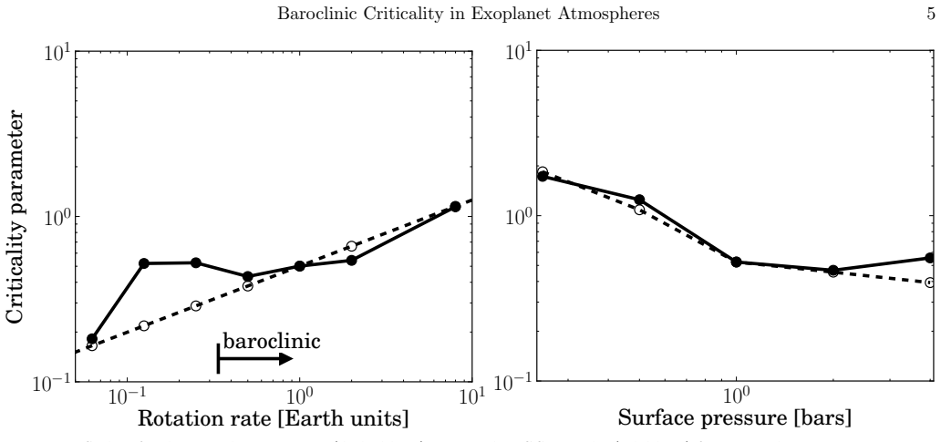
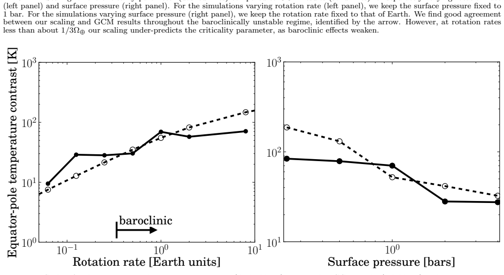
The central claim is that the baroclinic criticality parameter $\xi$—a measure of how slanted mid-latitude isentropes are, roughly the ratio of equator-to-pole to surface-to-tropopause potential temperature contrast—controls both heat transport and lapse rate, and that it scales as $\xi \propto (\Omega/\Omega_\oplus)^{2/5}(p/p_\oplus)^{-1/5}(H/H_\oplus)^{-3/5}(a/a_\oplus)^{3/5}(g/g_\oplus)^{-1/10}$. Combining this with the assumption that eddy heat flux is directed along isentropes yields equations (13) and (14), which predict the equator-to-pole potential temperature contrast and the bulk lapse rate (defined as the smaller of the surface-to-tropopause contrast and the contrast over one scale height) with no free parameters once the radiative-equilibrium contrast is fixed. The GCM comparisons show the equator-to-pole contrast increases with rotation rate and decreases with surface pressure, while the bulk lapse rate varies weakly and peaks near $\xi \approx 1$. The paper argues this confirms that baroclinic instabilities, not just radiative-convective balance, set the temperature structure of fast-rotating terrestrial exoplanets.
Load-bearing premise
The predictions inherit the assumption that eddy mixing follows the quasi-geostrophic turbulence law $D_{\mathrm{eddy}} \sim \beta (\xi L_d)^3$, with the Rhines scale tied to the deformation radius; if atmospheres with very different rotation or pressure mix according to a different law, the derived rotation and pressure exponents would not hold.
Editorial extensions
If this is right
- At fixed incident stellar flux, faster rotation widens the equator-to-pole potential temperature contrast, so fast rotators should have colder poles and larger sea-ice cover, an effect that could appear in orbital-phase albedo variations.
- The bulk lapse rate is only weakly dependent on planetary parameters near Earth-like values and peaks near $\xi \approx 1$; for rotation rates above about $8\Omega_\oplus$, further spin-up should reduce it rather than increase it.
- Spectroscopic retrievals that constrain the vertical temperature profile and tropopause height can directly test the predicted lapse rate, while full-phase thermal light curves can constrain the equator-to-pole contrast.
- The theory applies only to planets with active baroclinic instability, roughly those with rotation periods of about three days or shorter; slowly rotating and tidally locked planets require separate treatments.
- Extending the same reasoning to warm Jupiters and warm Neptunes is plausible, and the predicted increase of equator-to-pole contrast with rotation rate matches previous simulations of warm Jupiters.
Reading between the lines
- A retrieved equator-to-pole contrast alone would not pin down rotation rate or surface pressure, because the scalings depend on the combination $\xi \sim \Omega^{2/5} p^{-1/5}$ together with tropopause height, radius, and gravity; independent estimates of pressure or tropopause height would be needed to break the degeneracy.
- Because the theory fixes the radiative-equilibrium contrast $\Delta_h \theta_{eq}$ at one value, ice-albedo feedbacks are an unmodeled pathway; coupling the lapse-rate prediction to a sea-ice model might explain the anomalous ice-covered 2-4 bar cases noted in the paper.
- The predicted $\Omega^{2/5}$ exponent could be checked before exoplanet spectroscopy is ready, using existing dry dynamical-core GCMs or rotating-tank experiments that vary rotation rate over a wider range than the present suite.
- If the eddy-diffusivity closure survives, the same criticality balance may give testable predictions for the phase-curve amplitudes of fast-rotating gas giants as functions of their rotation rate and radiative timescale.
Signed reviews
Editorial analysis
A structured set of objections, weighed in public.
Referee Report
Summary. The manuscript derives scaling relations for the baroclinic criticality parameter, equator-to-pole potential temperature contrast, and bulk lapse rate of terrestrial exoplanet atmospheres. Building on Jansen & Ferrari (2013) and the Held-Larichev eddy-diffusivity closure, the authors obtain Equation (6) for the criticality parameter as a function of rotation rate, surface pressure, tropopause height, radius, and gravity, and then Equations (13) and (14) for the temperature contrast and lapse rate. The predictions are compared to ExoCAM GCM simulations with rotation rates from 0.0625 to 8 Earth values and surface pressures from 0.25 to 4 bars. The paper reports broad agreement for rotation rates greater than about one third of Earth's rotation rate and discusses observational tests of the scalings. Limitations of the theory for slowly rotating and tidally locked planets are acknowledged.
Significance. If the scalings hold, they provide compact, observationally relevant predictions for how the circulation of Earth-like exoplanets depends on basic planetary parameters. The paper connects a well-established body of geophysical fluid dynamics to exoplanet observations, and the GCM comparison is a reasonable and transparent test. The authors are honest about key inputs, such as the Earth-normalized criticality and the model-derived tropopause height and albedo, and they explicitly delimit the regime of applicability. The main weakness is that the validation is concentrated near the marginally critical regime, so the claim of applicability throughout the baroclinically unstable regime is not yet strongly supported.
major comments (3)
- [Section 2.1, Equations (5)-(6) and Figures 2-4] The exponents in Equations (6), (13), and (14) all inherit the Held-Larichev closure D_eddy ~ beta (xi L_d)^3 from Equation (5). The GCM comparisons test the integrated scaling rather than this closure directly, and the simulated runs lie mostly at or near xi ~ 1 (as noted in the discussion of Figure 4). Consequently, the paper's claim of applicability 'throughout the baroclinically unstable regime' rests largely on extrapolation to strongly supercritical states (xi >> 1) that the suite does not sample. I recommend adding a simulation or reanalysis at higher rotation rate or lower pressure that pushes xi well above 1, or substantially softening the scope claim to the near-critical regime.
- [Section 4.1, Figure 2 (right panel)] The pressure scaling is not a fully independent prediction because the predicted criticality uses the tropopause height H taken from the GCM experiments (the text states this explicitly). Since H enters Equation (6) with an exponent -3/5 and itself varies with surface pressure, the agreement between theory and model in Figure 2 partly reflects the model's H rather than a pure a priori prediction. The disclosure is appreciated, but the discussion should distinguish which parts of the pressure dependence are predicted and which are diagnosed, and should quantify the sensitivity to the choice of H (e.g., using a fixed H would change the predicted exponent to -1/5).
- [Section 4.2, Equation (13) and Figure 3] The fixed equilibrium equator-to-pole contrast Delta_h_theta_eq = 242 K is derived using an albedo of 0.55 taken from the Earth-like simulation, and the manuscript notes that albedo changes due to sea ice are ignored. For the 2 and 4 bar cases, which are ice-covered, the change in Delta_h_theta_eq is not accounted for and is invoked as the reason for the discrepancy. This is an acknowledged limitation, but it directly affects the pressure scaling that is a central target of the paper. Please estimate how Delta_h_theta_eq changes with the simulated albedo across the suite, so readers can judge how much of the apparent pressure trend in Figure 3 is attributable to the fixed Delta_h_theta_eq assumption.
minor comments (3)
- [Abstract] The word 'baroclincally' is a typo and should be 'baroclinically'.
- [Section 4.2, paragraph 1] The phrase 'there is no tunable parameter in our equations' is misleading because the theory is anchored by setting xi = xi_Earth for Earth-like parameters and by fixing Delta_h_theta_eq with an albedo taken from the model. These are inputs rather than tunable fits, but a more precise statement would acknowledge them as calibration choices.
- [Figure 2 caption] The caption refers to 'the arrow' but the figure does not visibly include an arrow in the rendered version; please either include the arrow in the figure or remove the reference.
Circularity Check
No significant circularity: the scaling theory is derived from stated closures and validated against GCMs without fitting the target outputs.
full rationale
The derivation chain is algebraic and self-contained: Eqs. (1)-(6) combine the Jansen-Ferrari criticality definition with the Held-Larichev eddy-diffusivity closure and the Showman-Guillot radiative-timescale scaling to produce Eq. (6); Eqs. (7)-(12) then derive the temperature-contrast scalings from a Newtonian-heating balance, with Eqs. (13)-(14) obtained by substitution. No step inverts a target output to define an input. The GCM comparison is not circular: ξ is measured from simulated isentropic slopes via Eq. (15), the theory is anchored by setting ξ=ξ_Earth at Earth parameters rather than fitting it, and the quoted statement in Sec. 4.2, 'there is no tunable parameter in our equations,' is accurate. The use of the model's albedo (0.55) to set Δhθeq=242 K and the use of GCM-computed tropopause heights in the pressure scaling are model-derived inputs, but they are diagnostics of the radiative state and geometry, not fits to the equator-to-pole contrast or bulk lapse rate being predicted; they do not force the predicted values, and the paper explicitly notes limitations (e.g., ignoring albedo changes with ice cover). The Jansen-Ferrari theory is prior work by a co-author, but it is an external, published theoretical result with stated assumptions that do not include the exoplanet scaling targets, so the self-citation is not load-bearing in a circular sense. Overall, no circular step is identifiable under the quoted-equation standard.
Assumptions & free parameters
free parameters (3)
- Earth criticality xi_Earth =
approximately 1
- Radiative equilibrium equator-to-pole contrast Delta_h_theta_eq =
242 K
- Tropopause height H for pressure scaling =
Taken from GCM for each surface pressure
assumptions (5)
- domain assumption Baroclinic instability dominates poleward heat transport in mid-latitudes of fast-rotating terrestrial planets.
- domain assumption Eddy diffusivity follows D_eddy ~ beta (xi L_d)^3 (Held and Larichev 1996).
- domain assumption Radiative relaxation timescale scales as tau_rad proportional to p/(g T^3).
- domain assumption Vertical radiative equilibrium contrast is negligible, Delta_v_theta_eq approximately 0.
- domain assumption Eddy heat flux is directed along isentropes, giving F_eddy,v ~ s F_eddy,h.
Cite this review
Pith. "Pith review of Scaling Relations for Terrestrial Exoplanet Atmospheres from Baroclinic Criticality." pith.science (2026). https://pith.science/paper/6EWOOGJQ
@misc{pith2026190802661,
  author       = {Pith},
  title        = {Pith review of: Scaling Relations for Terrestrial Exoplanet Atmospheres from Baroclinic Criticality},
  year         = {2026},
  howpublished = {\url{https://pith.science/paper/6EWOOGJQ}},
  note         = {Machine review of arXiv:1908.02661}
}
read the original abstract
The macroturbulent atmospheric circulation of Earth-like planets mediates their equator-to-pole heat transport. For fast-rotating terrestrial planets, baroclinic instabilities in the mid-latitudes lead to turbulent eddies that act to transport heat poleward. In this work, we derive a scaling theory for the equator-to-pole temperature contrast and bulk lapse rate of terrestrial exoplanet atmospheres. This theory is built on the work of Jansen & Ferrari (2013), and determines how unstable the atmosphere is to baroclinic instability (the baroclinic "criticality") through a balance between the baroclinic eddy heat flux and radiative heating/cooling. We compare our scaling theory to General Circulation Model (GCM) simulations and find that the theoretical predictions for equator-to-pole temperature contrast and bulk lapse rate broadly agree with GCM experiments with varying rotation rate and surface pressure throughout the baroclincally unstable regime. Our theoretical results show that baroclinic instabilities are a strong control of heat transport in the atmospheres of Earth-like exoplanets, and our scalings can be used to estimate the equator-to-pole temperature contrast and bulk lapse rate of terrestrial exoplanets. These scalings can be tested by spectroscopic retrievals and full-phase light curves of terrestrial exoplanets with future space telescopes.
Figures

Figures from the paper (1 more)

Reference graph
Works this paper leans on
-
[1]
2019, Publications of the Astronomical Society of the Pacific, 131, 064402
Baker, A., Blake, C., & Halverson, S. 2019, Publications of the Astronomical Society of the Pacific, 131, 064402
work page 2019
- [2]
-
[3]
Chai, J. & Vallis, G. 2014, Journal of the Atmospheric Sciences, 71, 2300
work page 2014
-
[4]
1947, Journal of Meteorology, 4, 135
Charney, J. 1947, Journal of Meteorology, 4, 135
work page 1947
- [5]
-
[6]
D., Seager, S., & Charbonneau, D
Wellnitz, D. D., Seager, S., & Charbonneau, D. 2009, The Astrophysical Journal, 700, 915
work page 2009
-
[7]
Cowan, N. B. & Strait, T. E. 2013, The Astrophysical Journal Letters, 765, L17
work page 2013
- [8]
Show all 58 references
-
[9]
2016, The Astrophysical Journal, 829, 52
Kreidberg, L., & Parmentier, V. 2016, The Astrophysical Journal, 829, 52
2016
-
[10]
2018, The Astronomical Journal, 155, 200
Feng, Y., Robinson, T., Fortney, J., Lupu, R., Marley, M., Lewis, N., Macintosh, B., & Line, M. 2018, The Astronomical Journal, 155, 200
2018
-
[11]
1979, Icarus, 40, 205
Gierasch, P., Ingersoll, A., & Pollard, D. 1979, Icarus, 40, 205
1979
-
[12]
2016, The Astrophysical Journal, 817, 17
Greene, T., Line, M., Montero, C., Fortney, J., Lustig-Yaeger, J., & Luther, K. 2016, The Astrophysical Journal, 817, 17
2016
-
[13]
2018, The Astrophysical Journal, 852, 67
Haqq-Misra, J., Wolf, E., Josh, M., Zhang, X., & Kopparapu, R. 2018, The Astrophysical Journal, 852, 67
2018
-
[14]
2000, in Program in Geophysical Fluid Dynamics (Woods
Held, I. 2000, in Program in Geophysical Fluid Dynamics (Woods
2000
-
[15]
& Hou, A
Held, I. & Hou, A. 1980, Journal of the Atmospheric Sciences, 37, 515
1980
-
[16]
& Larichev, V
Held, I. & Larichev, V. 1996, Journal of the Atmospheric Sciences, 53, 946
1996
-
[17]
& Ferrari, R
Jansen, M. & Ferrari, R. 2012a, Journal of the Atmospheric Sciences, 69, 695 —. 2012b, Journal of the Atmospheric Sciences, 70, 1456 —. 2013, Journal of the Atmospheric Sciences, 70, 2948
2013
-
[18]
Jansen, T., Scharf, C., Way, M., & Genio, A. D. 2019, The Astrophysical Journal, 875, 79
2019
-
[19]
& Flierl, G
Kaspi, Y. & Flierl, G. 2006, Journal of the Atmospheric Sciences, 64, 3177
2006
-
[20]
& Schneider, T
Kaspi, Y. & Schneider, T. 2011, Journal of the Atmospheric Sciences, 68, 2459 —. 2013, Journal of the Atmospheric Sciences, 70, 2596
2011
-
[21]
& Showman, A
Kaspi, Y. & Showman, A. 2015, The Astrophysical Journal, 804, 60
2015
-
[22]
& Fujii, Y
Kawahara, H. & Fujii, Y. 2010, The Astrophysical Journal, 720, 1333
2010
-
[23]
& Abbot, D
Koll, D. & Abbot, D. 2016, The Astrophysical Journal, 825, 99
2016
-
[24]
& Abbot, D
Komacek, T. & Abbot, D. 2019, The Astrophysical Journal, 871, 245
2019
-
[25]
2017, The Astrophysical Journal, 845, 5
Grimm, S., & Heng, K. 2017, The Astrophysical Journal, 845, 5
2017
-
[26]
2016, The Astrophysical Journal, 819, 84
Meadows, V., Terrien, R., & Mahadevan, S. 2016, The Astrophysical Journal, 819, 84
2016
-
[27]
& Loeb, A
Kreidberg, L. & Loeb, A. 2016, The Astrophysical Journal Letters, 832, L12
2016
-
[28]
& Showman, A
Lian, Y. & Showman, A. 2008, Icarus, 194, 597
2008
-
[29]
& Yung, Y
Line, M. & Yung, Y. 2013, The Astrophysical Journal, 779, 3
2013
-
[30]
2018, The Astronomical Journal, 156, 301
Fujii, Y., Luger, R., & Robinson, T. 2018, The Astronomical Journal, 156, 301
2018
-
[31]
& Seager, S
Madhusudhan, N. & Seager, S. 2009, The Astrophysical Journal, 707, 24
2009
-
[32]
& Brunini, A
Miguel, Y. & Brunini, A. 2010, Monthly Notices of the Royal Astronomical Society, 406, 1935
2010
-
[33]
& Snellen, I
Molliere, P. & Snellen, I. 2019, Astronomy & Astrophysics, 622, A139
2019
-
[34]
2017, The Astrophysical Journal, 850, 121
Fortney, J. 2017, The Astrophysical Journal, 850, 121
2017
-
[35]
2018, The Astrophysical Journal Letters, 858, L14
Olson, S., Schwieterman, E., Reinhard, C., Ridgewell, A., Kane, S., Meadows, V., & Lyons, T. 2018, The Astrophysical Journal Letters, 858, L14
2018
-
[36]
2010, Principles of Planetary Climate (Cambridge: Cambridge University Press)
Pierrehumbert, R. 2010, Principles of Planetary Climate (Cambridge: Cambridge University Press)
2010
-
[37]
2016, Nature Communications, 7, 10627
Popp, M., Schmidt, H., & Marotzke, J. 2016, Nature Communications, 7, 10627
2016
-
[38]
2017, The Astrophysical Journal, 846, 69
Rauscher, E. 2017, The Astrophysical Journal, 846, 69
2017
-
[39]
1975, Journal of Fluid Mechanics, 69, 417
Rhines, P. 1975, Journal of Fluid Mechanics, 69, 417
1975
-
[40]
2004, Journal of the Atmospheric Sciences, 61, 1317
Schneider, T. 2004, Journal of the Atmospheric Sciences, 61, 1317
2004
-
[41]
& Walker, C
Schneider, T. & Walker, C. 2006, Journal of the Atmospheric Sciences, 63, 1569
2006
-
[42]
& Guillot, T
Showman, A. & Guillot, T. 2002, Astronomy and Astrophysics, 385, 166
2002
-
[43]
2015, The Astrophysical Journal, 801, 95
Showman, A., Lewis, N., & Fortney, J. 2015, The Astrophysical Journal, 801, 95
2015
-
[44]
2015, Astronomy & Astrophysics, 576, A59
Snellen, I., de Kok, R., Birkby, J., Brandl, B., Brogi, M., Keller, C., Kenworthy, M., Schwarz, H., & Stuik, R. 2015, Astronomy & Astrophysics, 576, A59
2015
-
[45]
2001, Journal of the Atmospheric Sciences, 58, 3650
Sobel, A., Nilsson, J., & Polvani, L. 2001, Journal of the Atmospheric Sciences, 58, 3650
2001
-
[46]
1978, Journal of the Atmospheric Sciences, 35, 561
Stone, P. 1978, Journal of the Atmospheric Sciences, 35, 561
1978
-
[47]
2006, Atmospheric and Oceanic Fluid Dynamics: Fundamentals and Large-Scale Circulation (Cambridge: Cambridge University Press)
Vallis, G. 2006, Atmospheric and Oceanic Fluid Dynamics: Fundamentals and Large-Scale Circulation (Cambridge: Cambridge University Press)
2006
-
[48]
2015, The Astrophysical Journal, 802, 107
Waldmann, I., Tinetti, G., Rocchetto, M., Barton, E., Yurchenko, S., & Tennyson, J. 2015, The Astrophysical Journal, 802, 107
2015
-
[49]
2018, Quarterly Journal of the Royal Meteorological Society, 144, 2537
Wang, Y., Read, P., Tabataba-Vakili, F., & Young, R. 2018, Quarterly Journal of the Royal Meteorological Society, 144, 2537
2018
-
[50]
2017, The Astrophysical Journal Supplement Series, 231, 12
Tsigaridis, K. 2017, The Astrophysical Journal Supplement Series, 231, 12
2017
-
[51]
1978, Journal of the Atmospheric Sciences, 35, 1399 —
Williams, G. 1978, Journal of the Atmospheric Sciences, 35, 1399 —. 1979, Journal of the Atmospheric Sciences, 36, 932
1978
-
[52]
& Holloway, J
Williams, G. & Holloway, J. 1982, Nature, 297, 295
1982
-
[53]
2017, The Astrophysical Journal Letters, 839, L1
Wolf, E. 2017, The Astrophysical Journal Letters, 839, L1
2017
-
[54]
2017, The Astrophysical Journal, 837, 107
Wolf, E., Shields, A., Kopparapu, R., Haqq-Misra, J., & Toon, O. 2017, The Astrophysical Journal, 837, 107
2017
-
[55]
2015, The Astrophysical Journal, 806, 180
Wordsworth, R. 2015, The Astrophysical Journal, 806, 180
2015
-
[56]
2019, The Astrophysical Journal Letters, 876, L27
Yang, H., Komacek, T., & Abbot, D. 2019, The Astrophysical Journal Letters, 876, L27
2019
-
[57]
2014, The Astrophysical Journal Letters, 787, L2
Yang, J., Boue, G., Fabrycky, D., & Abbot, D. 2014, The Astrophysical Journal Letters, 787, L2
2014
-
[58]
2019, Icarus, 326, 225
Young, R., Read, P., & Wang, Y. 2019, Icarus, 326, 225
2019
Reviewed August 14, 2026 · model on record in the stance chip above.
Discussion (0). Continue with ORCID to comment.