REVIEW 4 major objections 4 minor 1 cited by
High dimensional parameter tuning for event generators
T0 review · 4 major / 4 minor · reviewed 2026-08-14 · deepseek-v4-flash
Pith's one-line read The Autotunes algorithm makes it practical to tune Monte Carlo event generators with 18–22 parameters by splitting the parameter space into correlated subspaces, weighting observables per sub-tune, and iterating the Professor method.
desk verdict A useful and honest extension of Professor tuning with a real algorithmic contribution, but the range-dependence of the chunking measure deserves a robustness check before the 'automatic' claim fully holds. read the letter →
The pith
A machine-rendered reading of the paper's core claim, the machinery that carries it, and where it could break.
The reading
What carries the argument
The central object is the normalized slope vector $\vec{N}_i$, one per observable bin $i$, obtained by linear regression of the normalized generator response on normalized parameters and then divided element-wise by the total slope vector $\vec{S}_N$. Its components encode which parameters influence which observables, and the shared normalization makes parameters that act on the same bins look correlated. $\vec{N}_i$ drives the whole pipeline: the chunking measure $M(\vec{J}) = \sum_i (\vec{N}_i\cdot\vec{J})^2$ picks the subspace $\vec{J}$ that maximizes the squared projection of the slope vectors, and the same vectors set the bin weights $w_i$ that enter the Professor $\chi^2$. The second essential piece is the iteration: the best 80% of the Professor runcombination fits define new parameter ranges, with a 20% margin, so each pass narrows the hyper-rectangle and improves the validity of the polynomial interpolation.
What would settle it
Run the full Autotunes pipeline on the same pseudo-data with two different but reasonable initial ranges and compare the recovered parameters; if the grouping flip shown in Appendix A alters the final tuned values by more than the quoted stability bands, the claim that the algorithm reliably identifies the right subspaces is falsified. The missing observation is whether range-induced grouping changes propagate into the final tune.
Extended reading notes
Core claim
On its own terms, the central claim is that high-dimensional event-generator tuning can be reduced to a sequence of low-dimensional Professor tunes by an algorithmic pre-processing step. Autotunes samples the parameter hyper-rectangle, normalizes parameter and observable ranges, and performs linear regressions to obtain a slope vector $\vec{S}_i$ for each observable bin $i$; each slope vector is divided component-wise by the summed slope vector $\vec{S}_N$ to give $\vec{N}_i$. The chunking measure $M(\vec{J})=\sum_i (\vec{N}_i\cdot\vec{J})^2$ selects, for a prescribed subspace dimension $n$, the set of parameters that should be tuned together, and the same $\vec{N}_i$ enter the observable weights $w_i=(\vec{N}_i\cdot\vec{J}_{\text{step}})^2/\sum_j N_i^j$ for each sub-tune. Tuning proceeds subspace by subspace with Professor's runcombination method, parameters from completed steps are held fixed, and the spread of the best fits defines narrowed ranges for the next iteration. In ideal polynomial tests the intended groupings are recovered; in the Pythia 8 pseudo-data test the iterated Autotunes method gives the smallest summed squared deviation from the true parameters; and in LEP tunes of 18 or 22 parameters the method yields stable values for the strong coupling $\alpha_S$ while flagging parameters the data barely constrain, such as the strange-quark fragmentation parameter $\mathtt{aExtraSQuark}$ and the shower cutoff $\mathtt{pTmin}$.
Load-bearing premise
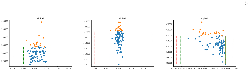
Changing the user-chosen initial ranges can flip which parameters are grouped together, even though the underlying generator is unchanged (the paper's Appendix A shows such a flip); the whole method therefore rests on the assumption that the initial ranges produce slope vectors that correctly identify which parameters belong together.
Editorial extensions
If this is right
- Retuning after a model change becomes a scripted pipeline rather than a manual expert exercise, because the subspace split and observable weights are produced algorithmically.
- Professor-based tuning extends from roughly ten parameters to the 18- and 22-parameter examples demonstrated here.
- Different hadronisation models can be tuned to the same data with the same algorithmic bias, making model comparisons less dependent on human tuning choices.
- A small number of iterations is enough: in the pseudo-data tests the second iteration visibly improves parameter recovery, with later iterations giving only minor changes.
- The per-parameter stability ranges produced by the runcombination spread identify which parameters the data actually constrain, such as the strong coupling, and which it leaves loose.
Reading between the lines
- The paper does not test whether the range-induced grouping flip documented in Appendix A changes the final tuned values; if it does, the algorithm's subspace split is not stable in the one place a user has control.
- The same slope-vector machinery could be repurposed to cluster observables and down-weight over-represented data, an extension the paper explicitly postpones; one could test whether that changes tunes on large LEP data sets.
- Because the generator is treated as a black box probed by random sampling, the method should carry over to other expensive simulators with many parameters, provided the polynomial approximation holds after range narrowing.
- A concrete next test is to weight merged higher-order samples as the paper suggests, suppressing observables dominated by perturbative uncertainties, and check whether the tuned strong coupling $\alpha_S$ shifts.
Signed reviews
Editorial analysis
A structured set of objections, weighed in public.
Referee Report
Summary. The paper proposes Autotunes, an iterative algorithm for tuning high-dimensional Monte Carlo event generator parameter spaces. The method first splits the full parameter space into lower-dimensional subspaces by maximizing a measure M built from range-normalized linear-regression slopes (Section III.A, Eq. 4), assigns per-observable weights from the same slope vectors (Section III.B, Eq. 5), runs Professor on each sub-tune, and then uses the spread of the best 80% of Professor run-combinations to define updated parameter ranges for the next iteration (Sections III.C and III.D). The algorithm is tested on polynomial pseudo-data, on Pythia 8 pseudo-data where it is compared with random and physics-motivated subgroupings, and on LEP data for Pythia 8, Herwig 7 with cluster hadronisation, and Herwig 7 with Pythia 8 string hadronisation. The paper concludes that the method enables semi-automatic tuning in spaces of 18 to 22 parameters and recovers pseudo-data parameters better than the two baselines.
Significance. If the central claim holds, the paper makes a useful practical contribution: event generator tuning is computationally expensive, and an automatic, reproducible way to split high-dimensional parameter spaces and iterate Professor-style tunes would benefit both generator development and phenomenological studies. The strengths of the paper are its concrete algorithmic formulation, the pseudo-data recovery tests with two baseline comparisons, and the honest discussion of range dependence in Appendix A. The method is not presented with formal guarantees, but the empirical comparison on Pythia 8 pseudo-data (Figure 4) is a meaningful step beyond a single idealized example. The main open question is whether the user-chosen initial ranges, through the chunking measure M, materially affect the final tuned values; the paper does not yet close this gap for the real-data tunes.
major comments (4)
- [Section III.A and Appendix A] The load-bearing chunking measure M(J)=sum_i (N_i dot J)^2 (Eq. 4) depends on the user-supplied initial hyper-rectangle through the range-normalized slopes N_i (Eq. 2). Appendix A demonstrates that changing the initial range for one parameter (Setup 3) flips the optimal grouping from (ClMaxLight, pTmin) plus (alphaS, gCM) to (ClMaxLight, gCM) plus (alphaS, pTmin). Since the subspace decomposition fixes both which parameters are tuned together and the weights in Eq. 5, this range dependence propagates through every sub-tune. The authors state that the weights are 'fairly stable if the same parameters are found to be correlated', but that conditional does not apply to the Setup 3 case, where the parameters found are not the same. No pseudo-data test is run with two different initial ranges that yield different groupings, so the paper does not establish whether later iterations erase the range dependence of the final tune. I would like the authors to either provide such a test, or explicitly qualify the claim that the method 'algorithmically' identifies the subspaces that should be tuned together.
- [Section V and Tables II-III] The real LEP tunes report only the tuned parameter values and their stability ranges; no chi-squared values, observable-level comparisons to the default tunes, or comparisons between the Autotunes result and a conventional Professor tune are given. Without any goodness-of-fit or distribution-level evidence, the statement that the method 'produces plausible LEP tunes' (Tables II and III) is not quantitatively supported. Please add, at minimum, the final chi-squared for each tune and a comparison of key observables (for example thrust, aplanarity, and charged multiplicity) against the defaults used as starting points.
- [Section IV.B and Figure 4(d)] The pseudo-data comparison in Figure 4(d) is the strongest evidence for the method, but the statement that 'the iterated Autotunes method improves the agreement' is only shown for a single random pseudo-data realization and three runs per baseline. The summed deviation metric is also not normalized per parameter, so the plot conflates the number of badly recovered parameters with the magnitude of deviations. I recommend reporting per-parameter deviations or a normalized chi-squared-like quantity, and, if computationally feasible, repeating the pseudo-data recovery for at least one additional random true parameter point to confirm that the advantage over the physically motivated baseline is not specific to one point.
- [Section III.B, Eq. (5)] The weight definition w_i = (N_i dot J_Step)^2 / sum_j N_j^i is central to the observable weighting, but it is not derived or justified beyond the heuristic sentence describing the numerator and denominator. In particular, the denominator sum_j N_j^i is not defined with explicit index ranges, and the reader cannot tell whether the sum runs over parameters of the current sub-tune or over all parameters. Please state the index ranges explicitly and give at least a short argument for why this particular normalization is preferable to alternatives such as normalizing the numerator by its maximum over bins.
minor comments (4)
- [General] The paper would benefit from a notation table or glossary; symbols such as Nsearch, the sub-tune dimension n, and the iteration count are introduced in the text but never collected in one place.
- [Section IV.A] In the polynomial test, the correlation matrices C_a are diagonal with entries k>1, so the 'correlated parameters' are actually parameters that independently enhance the same set of bins. Please clarify in the text that this is intended as a simplified model of correlation on the observable level and not a test of true multi-parameter correlations beyond the linear-regression sense used in the algorithm.
- [Appendix A, Figure 5] The caption of Figure 5 says 'The dashed lines correspond to Setup 2, which gives a same grouping of parameters as Setup 1', but Setup 2 also uses narrower ranges for two parameters; the text says Setups 1 and 2 give the same pairing, yet the figure shows Setup 1 and Setup 2 as dashed while Setup 3 is solid. Please make the caption and main text consistent about which setup is shown dashed and why.
- [Minor typographical issues] There are several typographical and formatting issues: 'first order approximation' in Section II.B should be 'first-order approximation'; 'runcombinations' is used without a hyphen or space in several places; the footnote about the implementation URL (gitlab.com/Autotunes) is not referenced in the text; and the sentence in Section IV.A 'As the result of each full tune serving as input to a next iteration' is grammatically incomplete.
Circularity Check
No significant circularity: the Autotunes method is validated against independent pseudo-data and real LEP data, and its chunking measure is a construction rather than a renamed fit of the target values.
full rationale
The paper's derivation chain is self-contained against external benchmarks. The chunking measure M(J)=Σ_i(N_i·J)^2 is built from linear-regression slopes of Monte Carlo samples over the user-defined hyper-rectangle; the target parameter values (in pseudo-data tests) and the measured LEP distributions (in real-data tunes) are not used to define M or the weights of Eq. (5), so there is no self-definitional reduction. The polynomial toy test uses observables of the same polynomial class that Professor interpolates, but the task is to recover randomly drawn coefficients, which is an independent target rather than an input to the algorithm. Reusing the same sampled points for subspace selection and for Professor fits is an in-sample statistical choice that could cause overfitting, but it does not make the predicted or tuned values equivalent to the inputs by construction. Appendix A documents that different initial ranges can flip the parameter grouping; that is a stability limitation and a correctness risk, not circularity. The cited Professor tool is external work, and the authors' own prior papers are used as background and tool references, not as a load-bearing uniqueness or derivation chain. Accordingly, no circular step meeting the required evidentiary standard is present.
Assumptions & free parameters
free parameters (5)
- Subspace dimension n
- Number of search points Nsearch =
not specified
- Polynomial order in Professor interpolation =
2
- Stability range cut =
80% of best runcombinations plus 20% margin
- Iteration count =
up to 4 in real tunes, up to 6 in the pseudo-data test
assumptions (6)
- domain assumption Professor's second-order polynomial is a sufficiently accurate surrogate for generator response within chosen parameter ranges.
- domain assumption Normalized linear-regression slopes N_i encode parameter influence and correlation on the observable level well enough to define good sub-spaces.
- domain assumption Observable bins are independent and the experimental uncertainties in Rivet and hepdata data can be treated as uncorrelated.
- domain assumption Pseudo-data generated at randomly chosen true parameter values is a valid benchmark for parameter recovery.
- ad hoc to paper Tuning subspaces in reverse order of M constrains globally important parameters first and improves convergence.
- ad hoc to paper The spread of the best 80% of Professor runcombinations measures tune stability and can define next-iteration ranges.
Cite this review
Pith. "Pith review of High dimensional parameter tuning for event generators." pith.science (2026). https://pith.science/paper/6WK5Y7DZ
@misc{pith2026190810811,
  author       = {Pith},
  title        = {Pith review of: High dimensional parameter tuning for event generators},
  year         = {2026},
  howpublished = {\url{https://pith.science/paper/6WK5Y7DZ}},
  note         = {Machine review of arXiv:1908.10811}
}
read the original abstract
Monte Carlo Event Generators are important tools for the understanding of physics at particle colliders like the LHC. In order to best predict a wide variety of observables, the optimization of parameters in the Event Generators based on precision data is crucial. However, the simultaneous optimization of many parameters is computationally challenging. We present an algorithm that allows to tune Monte Carlo Event Generators for high dimensional parameter spaces. To achieve this we first split the parameter space algorithmically in subspaces and perform a Professor tuning on the subspaces with bin wise weights to enhance the influence of relevant observables. We test the algorithm in ideal conditions and in real life examples including tuning of the event generators Herwig 7 and Pythia 8 for LEP observables. Further, we tune parts of the Herwig 7 event generator with the Lund string model.
Figures


Figures from the paper (2 more)


Forward citations
Cited by 1 Pith paper
-
Herwig 7 with the Lund String Model: Tuning and Comparative Hadronization Studies
A Lund string model tune inside Herwig 7, the LH Tune, gives competitive descriptions of many LEP and LHC observables and enables fixed-shower comparison of string vs cluster hadronization.
Reference graph
Works this paper leans on
-
[1]
Here, we require tree sub-tunes and performed four iterations
Tuning Herwig 7 with cluster model We retune the cluster-model with a 22 dimensional parameter space. Here, we require tree sub-tunes and performed four iterations. The results are listed in Appendix B. Comparing the results, we note that the method is in general able to find values outside of the given initial parameter ranges, see e.g. the αS(MZ) or the ...
-
[2]
Tuning Herwig 7 with Pythia 8 Strings The usual setup of the event generators are genuinely well-tuned and even though the tests of Section IV allow the conclusion that relatively arbitrary starting points lead to similar results, ignoring the previous knowledge completely seems undesirable. To create a real live example and further allow useful future st...
work page 2020
- [3]
- [4]
- [5]
- [6]
- [7]
-
[8]
T. Gleisberg, S. H¨ oche, F. Krauss, A. Schalicke, S. Schumann, and J.-C. Winter, JHEP 02, 056 (2004), hep-ph/0311263
arXiv 2004
Show all 41 references
-
[9]
Sj¨ ostrand, S
T. Sj¨ ostrand, S. Mrenna, and P. Z. Skands, JHEP05, 026 (2006), hep-ph/0603175
2006 arXiv
-
[10]
Sj¨ ostrand, S
T. Sj¨ ostrand, S. Ask, J. R. Christiansen, R. Corke, N. Desai, P. Ilten, S. Mrenna, S. Prestel, C. O. Rasmussen, and P. Z. Skands, Comput. Phys. Commun. 191, 159 (2015), 1410.3012
2015 arXiv
-
[11]
Reichelt, P
D. Reichelt, P. Richardson, and A. Siodmok, Eur. Phys. J. C77, 876 (2017), 1708.01491
2017 arXiv
-
[12]
Gieseke, P
S. Gieseke, P. Kirchgaeßer, and S. Pl¨ atzer, Eur. Phys. J.C78, 99 (2018), 1710.10906
2018 arXiv
- [13]
- [14]
- [15]
-
[16]
C. B. Duncan and P. Kirchgaeßer, Eur. Phys. J. C79, 61 (2019), 1811.10336
2019 arXiv
- [17]
-
[18]
Bewick, S
G. Bewick, S. Ferrario Ravasio, P. Richardson, and M. H. Seymour (2019), 1904.11866
2019 arXiv
-
[19]
Barate et al
R. Barate et al. (ALEPH), Phys. Rept. 294, 1 (1998)
1998
- [20]
-
[21]
Abreu et al
P. Abreu et al. (DELPHI), Z. Phys. C73, 11 (1996)
1996
-
[22]
P. Z. Skands, in Proceedings, 1st International Workshop on Multiple Partonic Interactions at the LHC (MPI08): Pe- rugia, Italy, October 27-31, 2008 (2009), pp. 284–297, 0905.3418, URL http://lss.fnal.gov/cgi-bin/find_paper.pl? conf-09-113
2009 arXiv
-
[23]
Buckley, H
A. Buckley, H. Hoeth, H. Lacker, H. Schulz, and J. E. von Seggern, Eur. Phys. J. C65, 331 (2010), 0907.2973
2010 arXiv
- [24]
- [25]
-
[26]
Ilten, M
P. Ilten, M. Williams, and Y. Yang, JINST 12, P04028 (2017), 1610.08328. 13 Parameter Def. Range H7+Dip.+Cluster H7+ ˜Q+ Cluster alphaS 0.126234 0.12 – 0.13 0.13008+0.00013 −0.00061 0.12455+0.00020 −0.00118 gConstituentMass 0.95 0.7 – 1.1 0.83+0.16 −0.07 1.0045+0.0028 −0.0006 ...
2017 arXiv
-
[27]
Buckley and H
A. Buckley and H. Schulz, Adv. Ser. Direct. High Energy Phys. 29, 281 (2018), 1806.11182
2018 arXiv
-
[28]
Bellm, S
J. Bellm, S. Pl¨ atzer, P. Richardson, A. Sidmok, and S. Webster, Phys. Rev. D94, 034028 (2016), 1605.08256
2016 arXiv
- [29]
-
[30]
Bothmann, M
E. Bothmann, M. Sch¨ onherr, and S. Schumann, Eur. Phys. J. C76, 590 (2016), 1606.08753
2016 arXiv
- [31]
- [32]
-
[33]
Maguire, L
E. Maguire, L. Heinrich, and G. Watt, J. Phys. Conf. Ser. 898, 102006 (2017), 1704.05473
2017 arXiv
-
[34]
Buckley, J
A. Buckley, J. Butterworth, L. Lonnblad, D. Grellscheid, H. Hoeth, J. Monk, H. Schulz, and F. Siegert, Comput. Phys. Commun. 184, 2803 (2013), 1003.0694
2013 arXiv
-
[35]
Andersson, G
B. Andersson, G. Gustafson, G. Ingelman, and T. Sj¨ ostrand, Phys. Rept. 97, 31 (1983)
1983
-
[36]
Sj¨ ostrand, Nucl
T. Sj¨ ostrand, Nucl. Phys.B248, 469 (1984)
1984
- [37]
- [38]
- [39]
-
[40]
Catani, B
S. Catani, B. R. Webber, and G. Marchesini, Nucl. Phys. B349, 635 (1991)
1991
-
[41]
Tanabashi et al
M. Tanabashi et al. (Particle Data Group), Phys. Rev. D98, 030001 (2018)
2018
Reviewed August 14, 2026 · model on record in the stance chip above.
Discussion (0). Continue with ORCID to comment.