REVIEW 4 major objections 5 minor 3 references
efunc: An Efficient Function Representation without Neural Networks
T0 review · 4 major / 5 minor · reviewed 2026-08-07 · deepseek-v4-flash
Pith's one-line read A $32^3$ grid with 13 floats per cell — softmax-weighted RBF-interpolated polynomial fields plus learned surface offsets — fits signed distance functions as accurately as million-parameter neural methods.
desk verdict A genuinely useful compact non-neural SDF representation with a clean parameterization and honest ablations, but the headline accuracy claim rests on thin single-run evidence and a load-bearing offset initialization whose sensitivity is untested. read the letter →
The pith
A machine-rendered reading of the paper's core claim, the machinery that carries it, and where it could break.
The reading
What carries the argument
The central machinery is the normalized RBF interpolation of polynomial Value functions on a regular grid, $O(q)=\sum_i \mathrm{softmax}(-\beta_i\|q-k_i\|^2) f(q-k_i;\phi_i)$, where $f$ is a truncated Taylor polynomial (degree one in the default setting) and $\beta_i$ is a learned inverse width. Each grid cell contributes a whole function rather than a scalar, and because the softmax weights have global support, every key contributes at every query, so no neighborhood search or hierarchical structure is needed. The second mechanism is the offset set $\{k_i+\Delta_i\}$, initially placed near the surface by mean shift, then learned, which adds local detail without changing the grid topology. Parameters are fitted with AdamW on mean squared error, and the forward and backward passes are fused into a single CUDA kernel that keeps only the softmax denominator from the forward pass, cutting memory from $\Theta(IJ)$ to $\Theta(J)$.
What would settle it
Fit the same nine test meshes with the $32^3\times 13$ representation with the mean-shift initialization disabled or fed corrupted surface samples, then measure near-surface Chamfer distance and Near-AE; a sharp degradation would confirm that the accuracy claim depends on external surface knowledge rather than on the RBF-polynomial form alone. Alternatively, compare against a hash-grid baseline under an equal parameter budget on a class of shapes whose ground-truth surfaces are not directly sampled, such as latent generative priors, where the offsets could not be initialized.
Extended reading notes
Core claim
The central claim is that replacing scalar grid values with polynomial functions and interpolating them with globally supported softmax-normalized radial basis weights yields an SDF representation whose approximation quality is comparable or superior to state-of-the-art neural, octree, and hash-grid representations at a small fraction of the parameter count. The argument is carried by the combined $O{+}\Delta$ representation of Eq. (16): one regular-grid RBF-polynomial field represents the bounding volume, and a second set of offset keys, initialized by mean shift on surface samples and updated during training, represents the near-surface region. The default configuration stores $32^3\times 13$ floats and achieves the best average Chamfer distance in the comparison. The paper further claims that the form is analytically differentiable, supports normal estimation through the gradient formula of Eq. (13), and permits direct grid-level shape manipulation.
Load-bearing premise
The method assumes that ground-truth surface points are available for the mean-shift initialization of the offset keys; when that initialization is removed, the paper's own ablation (Config-Full-3 versus Config-Full-4) shows near-surface absolute error roughly doubling, so noisy or missing surface samples would directly degrade accuracy.
Editorial extensions
If this is right
- SDF fitting can run on a plain regular grid of about 0.43M floats, matching or beating octree- and hash-grid neural methods in average Chamfer distance on the tested meshes.
- Surface normals follow from one analytic forward pass via Eq. (13), without finite differences or a separate network.
- Because the grid is regular and the weights are global, two shapes can be combined by splicing halves of their grids, a manipulation the paper demonstrates directly.
- The fused CUDA kernels cut training memory and time to roughly a tenth of a naive automatic-differentiation implementation, enabling training in about 16 MB at $32^3$ resolution on a desktop GPU.
- The same functional form composes with Fourier-cosine weights (Eq. 25) to decompose a shape into frequency bands, and the band-limited partial sums reconstruct the surface progressively.
Reading between the lines
- If the accuracy-per-parameter behavior carries to higher resolutions once kernel limits are lifted past $128^3$, this representation would be a natural latent-space prior for diffusion or autoregressive 3D generation, where per-shape codes must stay compact and differentiable.
- The global-support softmax weighting is mathematically the same shape as attention, so the representation could generalize to irregular or learned key sets such as point clouds or octree leaves without changing the loss; the paper does not explore that direction.
- The mean-shift initialization ties accuracy to a fixed sample of ground-truth surface points; a generative setting with latent geometry would need an amortized predictor for offsets, and the paper does not evaluate that regime.
- A direct extension would swap the polynomial Value for other analytic families such as trigonometric or exponential functions, potentially trading parameter count for frequency content on open or high-frequency surfaces; the paper leaves this untested.
Editorial analysis
A structured set of objections, weighed in public.
Referee Report
Summary. The paper introduces a non-neural signed distance function (SDF) representation called efunc, in which a normalized radial-basis-function weighted sum of polynomial functions is defined over a regular grid, augmented by learnable offset keys clustered near the surface. The authors derive analytic gradients, implement fused CUDA forward/backward kernels that reduce memory and time relative to automatic differentiation, and evaluate SDF fitting on nine meshes against FFN, NGLOD, Instant NGP, and DiF-Grid. The central empirical claim is that at 32^3×13 parameters (about 0.43M floats) the representation reaches Chamfer distance comparable to or better than MLP/octree/hash-grid baselines that use an order of magnitude more parameters. The paper also presents a taxonomy of function representations, ablations, and applications to frequency decomposition, normal estimation, and shape manipulation.
Significance. If the empirical claims hold, the compact explicit representation is a useful alternative to neural SDFs for applications needing fast analytic gradients, low memory, and interpretable grid structure. The paper's strengths are the algebraically correct gradient derivations (Eqs. 13–14 and 20–22), the complete forward/backward algorithms that are implementable from the text, and an order-of-magnitude reduction in memory compared to a naive PyTorch implementation. The proposed framework taxonomy in Section 2 is a clearly presented contribution that situates the method among classical and neural representations. The principal weakness is that the headline comparison rests on single-run Chamfer values on nine meshes and on a mean-shift initialization whose sensitivity is not examined; these gaps need to be addressed before the 'comparable or superior' claim can be considered established.
major comments (4)
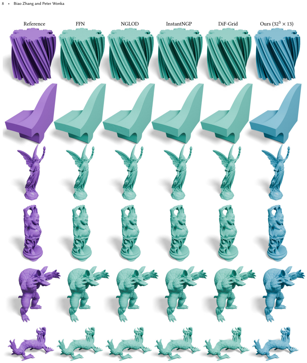
- [§4.2, Table 3] The central claim of 'comparable or superior performance' is not statistically supported. Each entry is a single run on one mesh, with no error bars, no repeated-seed results, and no significance test. The mean Chamfer distances separating Ours (32^3×13, 9.227) from NGLOD (9.273) and I-NGP (9.288) are far smaller than the per-shape variations and likely within noise. Please report means and standard deviations over at least three independent optimization runs (or across sampling seeds for the 100k-point Chamfer evaluation) and state whether the differences are significant.
- [§3.3, Eq. (17), Table 4] The mean-shift initialization is a load-bearing component whose robustness is untested. Config-Full-4 with initialization improves Near-AE from 6.499 to 3.772 and Near-IOU from 95.218 to 97.119 relative to Config-Full-3 under the same parameter budget. The paper fixes N=16,384 ground-truth surface points and bandwidth 100 'in almost all experiments' without varying N, perturbing the surface samples, or testing noisy input. Because the method is advertised for SDF fitting in general and for future generative use, the sensitivity of near-surface accuracy to the quantity and quality of surface points should be quantified; otherwise the reported near-surface advantage is only known to hold for clean, dense mesh samples.
- [§4.2, Table 3 and Conclusion] The claim of 'significantly fewer parameters while achieving comparable approximation quality' is overstated relative to the evidence across resolutions. At 16^3×13 parameters the mean Chamfer distance is 9.659, which is worse than all four neural baselines (9.39–9.37); only the 32^3 grid is comparable or slightly better. The paper should scope the claim to the tested 32^3 resolution and, ideally, report a parameter-accuracy curve showing the resolution at which parity with each competitor is reached.
- [§4.4, Eq. (25)] The function-decomposition application is not reproducible as written because Eq. (25) uses cos(b·π·q) with q∈R^3, but the expression is written as if q were a scalar. Please specify whether the cosine is applied per coordinate (and how the resulting vector is reduced to a scalar S(q)), and reconcile the statement that each O_b uses 16^3×4 floats with the total of 20480×B parameters, which appears to include the scale parameter β.
minor comments (5)
- [Table 4] The label 'mesh-shift initialization' appears to be a typo for 'mean-shift initialization'.
- [§3.3, Eq. (17)] Please state where the N=16,384 surface points are sampled from (e.g., uniformly on the ground-truth mesh or from a dense point cloud) and provide a rationale or sensitivity check for the fixed bandwidth 100.
- [§4.1] The experimental protocol should state the number of training iterations, the random seed for point sampling, and the hardware used, since the reported 20-minute training time is not directly comparable to the competitor timings cited in the limitation paragraph.
- [§4.2, first paragraph] The sentence 'Our results are getting better when the resolution is increased' is informal for a journal; please rephrase.
- [§3.1] In Eq. (9) the parameter vector is written as θ={k_i,β_i,v_i}∈R^{R×R×R×2}, but the keys k_i are grid points and the expression omits the keys' coordinates; please clarify which entries are trainable and which are fixed.
Circularity Check
No significant circularity: efunc is an empirical fitting method evaluated on the same-shape benchmark, and the mean-shift offset initialization is a data-dependent optimization aid, not a fitted parameter disguised as a prediction.
full rationale
The paper's derivation chain is a parametric representation plus an optimization objective: Eq. (11)/(16) define the proposed SDF field, Eq. (18) defines the MSE loss against ground-truth point-distance pairs, and Tables 3 and 4 report reconstruction and approximation errors on those shapes. Because the task is fitting, matching the training signal is the goal rather than a circular prediction. The mean-shift offset initialization in Eq. (17) uses N=16384 ground-truth surface points, and Table 4 (Config-Full-3 vs Config-Full-4) shows it materially improves Near-AE and Near-IOU; however, this is an initialization that changes the starting point of optimization, and the reported metrics evaluate the final optimized field, not the initialization itself. No claimed prediction is defined in terms of the fitted parameters, and no parameter is fit to a subset of data and then reported as a prediction of a closely related quantity. Section 2's framework is a taxonomy of existing work, not a load-bearing derivation. The self-citations (Zhang et al. 2022, 2023) appear only as examples of global interpolation in the framework and are not used to justify the validity of the proposed method. There is no imported uniqueness theorem, no ansatz smuggled in through citation, and no renaming of a known result presented as a derivation. The limitation section notes speed and GPU-architecture constraints rather than any circular dependency. The lack of sensitivity analysis for the number or noise level of surface samples is a robustness and generalization gap, but it is not a circularity defect.
Assumptions & free parameters
free parameters (6)
- RBF sharpness beta_i per key =
learned, initialized to exp(7) ~ 1096
- Polynomial coefficients phi_i (degree 1: 4 per key per side) =
learned
- Offset vectors Delta_i =
learned, initialized by mean shift
- Grid resolution R (default 32) =
32
- Polynomial degree (default 1) =
1
- Mean-shift bandwidth (100 in Eq. 17) =
100
assumptions (4)
- standard math SDFs are smooth enough to be locally approximated by low-order polynomials (Taylor's theorem).
- standard math The softmax-normalized RBF weighting (Nadaraya-Watson kernel regression) gives a valid, smooth partition of unity.
- domain assumption AdamW optimization of the non-convex MSE loss converges to a useful local minimum.
- domain assumption Ground-truth surface points are available for mean-shift initialization and are representative of the target surface.
Cite this review
Pith. "Pith review of efunc: An Efficient Function Representation without Neural Networks." pith.science (2026). https://pith.science/paper/6YZYMCKZ
@misc{pith2026250521319,
  author       = {Pith},
  title        = {Pith review of: efunc: An Efficient Function Representation without Neural Networks},
  year         = {2026},
  howpublished = {\url{https://pith.science/paper/6YZYMCKZ}},
  note         = {Machine review of arXiv:2505.21319}
}
read the original abstract
Function fitting/approximation plays a fundamental role in computer graphics and other engineering applications. While recent advances have explored neural networks to address this task, these methods often rely on architectures with many parameters, limiting their practical applicability. In contrast, we pursue high-quality function approximation using parameter-efficient representations that eliminate the dependency on neural networks entirely. We first propose a novel framework for continuous function modeling. Most existing works can be formulated using this framework. We then introduce a compact function representation, which is based on polynomials interpolated using radial basis functions, bypassing both neural networks and complex/hierarchical data structures. We also develop memory-efficient CUDA-optimized algorithms that reduce computational time and memory consumption to less than 10% compared to conventional automatic differentiation frameworks. Finally, we validate our representation and optimization pipeline through extensive experiments on 3D signed distance functions (SDFs). The proposed representation achieves comparable or superior performance to state-of-the-art techniques (e.g., octree/hash-grid techniques) with significantly fewer parameters.
Figures


Figures from the paper (10 more)




Reference graph
Works this paper leans on
-
[2003]
Multi-level partition of unity implicits. ACM Trans. Graph. 22, 3 (July 2003), e𝑓 unc: An Efficient Function Representation without Neural Networks • 13 463–470. https://doi.org/10.1145/882262.882293 Jeong Joon Park, Peter Florence, Julian Straub, Richard Newcombe, and Steven Love- grove. 2019. Deepsdf: Learning continuous signed distance functions for sh...
arXiv 2019
-
[2020]
Convolutional occupancy networks. In Computer Vision–ECCV 2020: 16th Eu- ropean Conference, Glasgow, UK, August 23–28, 2020, Proceedings, Part III 16 . Springer, 523–540. Xuanchi Ren, Jiahui Huang, Xiaohui Zeng, Ken Museth, Sanja Fidler, and Francis Williams. 2024. Xcube: Large-scale 3d generative modeling using sparse voxel hierarchies. In Proceedings of...
work page 2020
-
[2024]
GALA: Geometry-Aware Local Adaptive Grids for Detailed 3D Generation
GALA: Geometry-Aware Local Adaptive Grids for Detailed 3D Generation. arXiv preprint arXiv:2410.10037 (2024). Lior Yariv, Omri Puny, Oran Gafni, and Yaron Lipman. 2024. Mosaic-sdf for 3d generative models. In Proceedings of the IEEE/CVF Conference on Computer Vision and Pattern Recognition. 4630–4639. Biao Zhang, Matthias Nießner, and Peter Wonka. 2022. 3...
work page Pith review arXiv 2024
Reviewed August 7, 2026 · model on record in the stance chip above.
Discussion (0). Sign in to comment.