REVIEW 4 major objections 5 minor 47 references
Steady states of non-axial dipolar rods driven by rotating fields
T0 review · 4 major / 5 minor · reviewed 2026-08-14 · deepseek-v4-flash
Pith's one-line read A two-dimensional system of magnetic rods with tilted dipoles, driven by a rotating field, has three steady states—dynamic aggregates, an isotropic fluid, and a clustered fluid—whose location in the $B$–$\omega$ plane is set by the…
desk verdict A useful parameter scan of rotating-field-driven dipolar rods; the three-state phase diagram is credible, but the synchronization order parameter is not independently validated and the quantitative support is thinner than the abstract suggests. read the letter →
The pith
A machine-rendered reading of the paper's core claim, the machinery that carries it, and where it could break.
The reading
What carries the argument
The load-bearing object is the single-rod dipole autocorrelation function $C_\mu(t) = \frac{1}{N}\langle \sum_i \hat{\mu}_i(t)\cdot \hat{\mu}_i(0)\rangle$, a time-series measure of how much each rod's dipole direction at time $t$ remembers its direction at time $0$. Its power comes from the exact identity for phase-locked rods, $C_\mu(t) = \frac{n_s}{N}\cos(\omega t)$ (Eq. 18), which turns the oscillation amplitude into a synchronization count. Paired with the time-averaged potential for in-phase dipoles, $\bar{u}_D(r) = -\mu^2/(2r^3)$, the machinery explains why synchronized rods attract isotropically and form dynamic aggregates, while unsynchronized rods are left to their bare anisotropic rod-rod forces and cluster into chain-like or ribbon-like structures.
What would settle it
Tag each rod's instantaneous phase relative to the rotating field in the same simulations, count the rods whose phase difference stays below a small threshold over many periods, and compare that direct count with the amplitude of $C_\mu(t)$. If the direct count disagrees with $n_s/N$ by more than numerical noise, the $0.65$ threshold used to define dynamic aggregates is an artifact of the amplitude interpretation.
Extended reading notes
Core claim
The central discovery, on the paper's own terms, is that the synchronization fraction is the organizing quantity of the phase diagram. For a population rotating perfectly in phase, the dipole autocorrelation satisfies $C_\mu(t) = \frac{n_s}{N}\cos(\omega t)$, so the amplitude of the time series is literally the fraction $n_s/N$ of rods locked to the field. The paper uses that amplitude to separate regimes: dynamic aggregates are found for $n_s/N \gtrsim 0.65$; the isotropic fluid shows either a smaller oscillation amplitude or a damped, non-oscillatory decay; and the clustered fluid shows a monotonic stretched-exponential decay whose relaxation time grows with polymerization. The tilt angle $\Psi$ matters because it changes the preferred pair bond from head-to-tail at small $\Psi$ to ribbon-like at large $\Psi$, shifting where the phase boundaries sit in the $B$-$\omega$ plane.
Load-bearing premise
The argument depends on assuming that the amplitude of the dipole autocorrelation function counts synchronized rods exactly: every locked rod contributes $\cos(\omega t)$ and every unlocked rod contributes zero on average.
Editorial extensions
If this is right
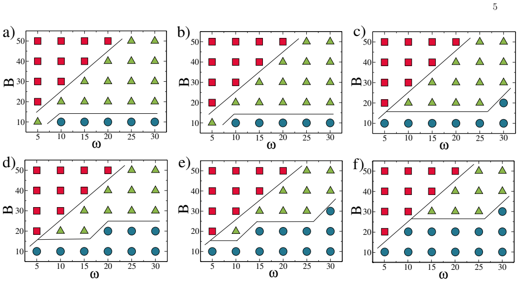
- At fixed $B$, increasing $\omega$ moves the system from the high-synchronization dynamic-aggregate state toward the isotropic fluid and then the clustered fluid, so the rotation frequency alone can drive the system across the phase diagram.
- Because the amplitude of $C_\mu(t)$ identifies the dynamic-aggregate state at $n_s/N \gtrsim 0.65$, the aggregate regime can in principle be detected from autocorrelation time-series data without computing cluster structure.
- The clustering in the low-synchronization regime relaxes through a stretched exponential with exponent $\beta<1$, meaning rotational relaxation is non-exponential and slows as polymerization $\Phi$ increases.
- The tilt angle $\Psi$ selects the internal bond geometry, head-to-tail for small $\Psi$ and ribbon-like for large $\Psi$, so the same field protocol produces different cluster architectures when the dipole is more misaligned.
- In the limit of full synchronization the rod-rod interaction is the isotropic attraction $\bar{u}_D = -\mu^2/(2r^3)$, so dynamic aggregates can be understood as an effective equilibrium cluster phase even though the system is driven.
Reading between the lines
- A direct per-rod phase-lag measurement in the same simulations could test whether the $\approx 0.65$ amplitude threshold is a genuine synchronization threshold or a convenient correlation envelope; if it is only an envelope, the phase boundaries would shift when synchronization is counted rod by rod.
- The identity $C_\mu(t) = (n_s/N)\cos(\omega t)$ should apply to any periodic field protocol whose locked rods follow the same in-phase form, so the same analysis could be carried over to precessing or pulsed fields.
- The reentrant clustering seen at $\Psi=45^{\circ}$, with clusters at low and high $\omega$ but chains at intermediate $\omega$, suggests the effective rod-rod interaction is non-monotonic in synchronization; a fine sweep of $\Psi$ could test whether the reentrance tracks the crossover from head-to-tail to ribbon-like bonding.
- Because the dynamic aggregate is governed by an isotropic attractive potential, its cluster-size statistics might obey equilibrium scaling laws for the effective coupling; the paper does not test this.
Signed reviews
Editorial analysis
A structured set of objections, weighed in public.
Referee Report
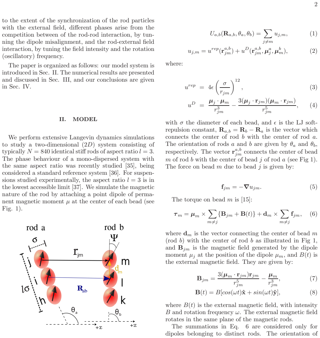
Summary. This manuscript reports Langevin dynamics simulations of a two-dimensional system of rigid magnetic rods, each modeled as three aligned soft beads with a central point dipole tilted by an angle Psi relative to the rod axis. The rods are driven by a rotating magnetic field of amplitude B and frequency omega. The authors classify the steady states into three regimes: dynamic aggregates, isotropic fluid, and clustered fluid, and present B-omega phase diagrams for Psi = 15 to 90 degrees. The classification is based on visual inspection of configurations, the pair correlation function g(r), the polymerization Phi, and the single-dipole autocorrelation function C_mu(t). The central quantitative relation is Eq. (18), C_mu(t) = (ns/N) cos(omega t), whose oscillation amplitude is interpreted as the fraction of rods synchronized with the field. Figure 10 uses this amplitude to claim that dynamic aggregates occur for ns/N greater than about 0.65. The conclusions frame the three phases as consequences of high, intermediate, and low synchronization regimes.
Significance. If the central claims hold, the work provides a useful descriptive phase diagram for a experimentally motivated class of anisotropic magnetic colloids under rotating fields, and it identifies a simple dynamical observable, C_mu(t), as a candidate order parameter for synchronization. The model and simulation protocol are conventional and the three-state picture is plausible and worth reporting. The paper also makes a concrete, falsifiable prediction: the boundaries of the dynamic-aggregate regime coincide with an oscillation amplitude of C_mu(t) above about 0.65. However, the quantitative support for this prediction is not yet established, because Eq. (18) is not validated against an independent measure of synchronization and the phase boundaries in Fig. 3 are hand-drawn guides without statistical uncertainties. With the requested additions, the paper would be a solid contribution to the soft-matter literature.
major comments (4)
- [Sec. III B, Eq. (18)] The derivation of C_mu(t) = (ns/N) cos(omega t) is not secure. A rod whose dipole rotates at the field frequency with a constant phase lag delta, mu_hat(t) = cos(omega t - delta) x_hat + sin(omega t - delta) y_hat, gives mu_hat(t) dot mu_hat(0) = cos(omega t), independent of delta. Therefore the oscillation amplitude of C_mu(t) counts all frequency-locked rods, not only rods with zero phase lag as stated in the text. In addition, rods that are not frequency-locked do not contribute zero: a rod with a fixed orientation contributes a non-oscillatory positive value near unity at short times, and a slowly reorienting rod contributes a decaying background. The paper does not specify how the oscillation amplitude in Fig. 10 is separated from this background, nor does it validate Eq. (18) against an independent measure such as the distribution of phase differences phi_i(t) = arg(mu_i(t)) - omega t or a complex order parameter. Because the dynamic-aggregate regime is defined by ns/N greater than about 0.65, this mapping is load-bearing and needs separate verification.
- [Sec. III A, Fig. 3] The B-omega phase boundaries are drawn as guides for the eyes, and the symbols are assigned by visual inspection of configurations and g(r). The manuscript does not report error bars, the number of independent runs, or a quantitative classification protocol (for example, a threshold in polymerization, cluster-size distribution, or synchronization order parameter). Without such a protocol, the phase diagram is not reproducible and the claim of three distinct steady states is not quantitatively established.
- [Table I] The polymerization values in Table I show a strong non-monotonic dependence on omega, e.g., for Psi = 60 degrees and B = 20, Phi = 0.909 at omega = 5, 0.245 at omega = 10, 0.351 at omega = 15, and 0.968 at omega = 20, with no error bars. The manuscript does not state whether these variations are statistically significant or whether they correspond to the phase boundaries in Fig. 3. This leaves the relationship between polymerization and the phase classification unclear.
- [Sec. III A, bond definition] The bond criterion of shortest bead separation less than or equal to 1.4 sigma is extracted from the pair-minimum distances at Psi = 15 and 90 degrees and then applied to all Psi and to many-body clusters. The global minimum of the pair interaction shifts with Psi, so it is not obvious that a single cutoff is valid for intermediate angles or inside clusters. Since Phi and the statement that clustered fluids consist of bonded rods depend on this criterion, its generalization should be justified or replaced by a Psi-dependent bond definition.
minor comments (5)
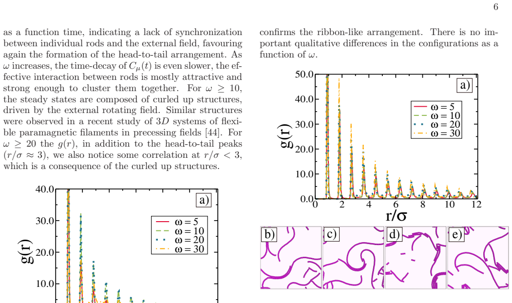
- [Sec. III B, text near Fig. 8] The text says 'less than 40% of the rods are in phase with the external field [Fig. 8(a)]', but Fig. 8(a) shows g(r); the relevant autocorrelation data are in Fig. 9(a). The figure reference appears to be incorrect.
- [Throughout] The manuscript uses both 'Dynamic aggregates' and 'Dynamical aggregates' for the same phase. The nomenclature should be made consistent.
- [Fig. 10] The caption calls the plotted quantity the 'critical amplitude of oscillation', but the figure shows measured amplitudes for the dynamic-aggregate phase and no error bars. A definition of 'critical' and the uncertainty in the 0.65 threshold should be provided.
- [Sec. III B, Eq. (19)] The stretched exponential fit parameters tau and beta are shown only in the legend boxes of Fig. 12. Reporting them in a table would allow readers to compare relaxation times quantitatively.
- [Sec. II, reduced units] The reduced frequency is defined as omega* = omega / sqrt(epsilon^{-1} M sigma^2), but the notation is ambiguous because omega is used both for the angular frequency of the field and for the angular velocity of rods. Clarifying the notation would improve readability.
Circularity Check
No significant circularity: the phase diagram is built from configurations and g(r), independent of the synchronization observable; Eq. (18) is a diagnostic mapping with a phase-lag caveat, not a self-referential derivation.
full rationale
The paper's central result is a B-omega-Psi classification of steady states (Fig. 3), which is obtained from visual inspection of configurations and from the pair correlation function g(r) (Eq. 14), together with a bond-length criterion. These phase labels do not depend on C_mu(t). The synchronization observable is introduced afterward (Sec. III B) and used to characterize the already identified phases; the abstract and conclusions describe dynamic aggregates, isotropic fluid, and clustered fluid as configurations, with synchronization regimes invoked as an explanatory correlate, not as the classifier. The threshold ns/N ~ 0.65 is a descriptive summary of the dynamic-aggregate points already labeled in Fig. 10, not a fitted parameter used to predict those labels. The derivation of Eq. (18) assumes perfectly in-phase rotation, Eq. (17); this is a validity limitation (constant phase-lagged rods also contribute cos(omega t), and unsynchronized rods give a decaying background), but it is not circular: the observable amplitude is not the input from which the phase diagram is derived. The model self-citations [15,22] provide the peapod/DSS simulation method, not the claimed phase diagram, and are not used as a uniqueness or enabling theorem. No step reduces a predicted quantity to a fitted input by construction.
Assumptions & free parameters
free parameters (2)
- Bond cutoff delta_c =
1.4 sigma
- Synchronization threshold ns/N =
~0.65
assumptions (4)
- domain assumption Langevin dynamics with Stokes friction and Gaussian white noise is a valid model for the colloidal rods, using friction coefficients from Refs. [38,39].
- domain assumption When dipoles are synchronized with the rotating field, the time-averaged dipolar pair potential is -mu^2/(2 r^3) (Eq. 13).
- domain assumption The simulation box is large enough that direct truncation of r^-3 dipolar interactions is sufficient, without long-range summation techniques.
- ad hoc to paper The pair-minimum separation of 1.4 sigma for isolated rods at Psi=15 and 90 degrees applies to all Psi and to many-body clusters.
Cite this review
Pith. "Pith review of Steady states of non-axial dipolar rods driven by rotating fields." pith.science (2026). https://pith.science/paper/7AO2TYND
@misc{pith2026190806718,
  author       = {Pith},
  title        = {Pith review of: Steady states of non-axial dipolar rods driven by rotating fields},
  year         = {2026},
  howpublished = {\url{https://pith.science/paper/7AO2TYND}},
  note         = {Machine review of arXiv:1908.06718}
}
read the original abstract
We investigate a two-dimensional system of magnetic colloids with anisotropic geometry (rods) subjected to an oscillating external magnetic field. The structural and dynamical properties of the steady states are analyzed, by means of Langevin Dynamics simulations, as a function of the misalignment of the intrinsic magnetic dipole moment of the rods with respect to their axial direction, and also in terms of the strength and rotation frequency of an external magnetic field. The misalignment of the dipole relative to their axial direction is inspired by recent studies, and this is extremely relevant in the microscopic aggregation states of the system. The dynamical response of the magnetic rods to the external magnetic field is strongly affected by such a misalignment. Concerning the synchronization between the magnetic rods and the direction of the external magnetic field, we define three distinct regimes of synchronization. A set of steady states diagrams are presented, showing the magnitude and rotation frequency intervals in which the distinct self-organized structures are observed.
Figures

Figures from the paper (8 more)




Reference graph
Works this paper leans on
-
[1]
C. S. Dias, N. A. M. Araujo, M. M. Telo da Gama, Phys- ical Review E 87, 3 (2013)
work page 2013
-
[2]
D. M. Rutkowski, O. D. Velev, S. H. Klapp, and C. K. Hall,Soft matter , 13, 17 (2017)
work page 2017
-
[3]
T. Heinemann, M. Antlanger, M. Mazars, S. H. Klapp, and G. Kahl, The Journal of chemical physics , 144, 7 (2016)
work page 2016
-
[4]
Nisisako, T., Current Opinion in Colloid & Interface Sci- ence 25, 1 (2016)
work page 2016
-
[5]
Daddi-Moussa-Ider, Abdallah and Menzel, Andreas M., Physical Review Fluids 3, 9 (2018)
work page 2018
-
[6]
T. Debnath, Y. Li, P. K. Ghosh, and F. Marchesoni, Physical Review E , 97, 4 (2018)
work page 2018
- [7]
-
[8]
Crocker, Phys- ical review letters 120, 11 (2018)
Mehdi Molaei, Ehsan Atefi, and John C. Crocker, Phys- ical review letters 120, 11 (2018)
work page 2018
Show all 47 references
-
[9]
Stoeva,Fengwei Huo,Jae-Seung Lee, and, Chad 10 A
Savka I. Stoeva,Fengwei Huo,Jae-Seung Lee, and, Chad 10 A. Mirkin, Journal of the American Chemical Society 127, 44 (2005)
2005
-
[10]
Howes, Rona Chandrawati, and Molly M
Philip D. Howes, Rona Chandrawati, and Molly M. Stevens, Science 346, 6205 (2014)
2014
-
[11]
Fabrice Cousin, Valrie Cabuil, and Pierre Levitz, Lang- muir 18, 5 (2002)
2002
-
[12]
Gubin, Magnetic Nanoparticles, Wiley (2009)
S. Gubin, Magnetic Nanoparticles, Wiley (2009)
2009
-
[13]
B. J. Lemaire, P. Davidson, J. Ferr, J. P. Jamet, P. Pa- nine, I. Dozov and J. P. Jolivet, Physical review letters 88, 12 (2002)
2002
-
[14]
Philip, P
J. Philip, P. Shima and B. Raj, Applied Physics Letters 91, 203108 (2007)
2007
-
[15]
Jorge L. C. Domingos, F.M. Peeters, W.P. Ferreira, Phys- ical Review E 96, 1 (2017)
2017
-
[16]
C. E. Alvarez and S. H. Klapp, Soft Matter 8, 7480 (2012)
2012
-
[17]
Abrikosov, S
A.I. Abrikosov, S. Sacanna, A.P. Philipse, P. Linse, Soft Matter 9, 37 (2013)
2013
-
[18]
Yener, S.H
A.B. Yener, S.H. Klapp, Soft Matter 12, 7 (2016)
2016
-
[19]
Martinez-Pedrero, A
F. Martinez-Pedrero, A. Cebers, and P. Tierno, Phys. Rev. Applied 6, 034002 (2016)
2016
-
[20]
Singh H, Laibinis PE, Hatton TA., Langmuir 21, 24 (2005)
2005
-
[21]
Lee, and C.M
S.H. Lee, and C.M. Liddell, Small 5, 17 (2009)
2009
-
[22]
Jorge L. C. Domingos, F. M. Peeters, W. P. Ferreira, PloS One 13, e0195552 (2018)
2018
-
[23]
Carrey, and N
J. Carrey, and N. Hallali, Phys. Rev. B 94, 184420 (2016)
2016
-
[24]
Birringer, H
R. Birringer, H. Wolf, C. Lang, A. Tsch¨ ope and A. Michels, Zeitschrift f¨ ur Physikalische Chemie222, 229 (2008)
2008
-
[25]
N. Coq, S. Ngo, O. du Roure, M. Fermigier and D. Bar- tolo, Physical Review E 82, 041503 (2010)
2010
-
[26]
P. Dhar, C. D. Swayne, T. M. Fischer, T. Kline and S. Ayusman, Nano Lett. , 7, 1010 (2007)
2007
-
[27]
W. A. Shelton, K. D. Bonin and T. G. Walker, Physical Review E 71, 036204 (2005)
2005
-
[28]
J. E. Martin, R. A. Anderson and C. P. Tigges, J. Chem. Phys. 108, 7887 (1998)
1998
-
[29]
J. E. Martin, R. A. Anderson and C. P. Tigges, J. Chem. Phys., , 110, 4854 (1999)
1999
-
[30]
Elsner, C
N. Elsner, C. P. Royall, B. Vincent and D. R. E. Snoswell, J. Chem. Phys. 130, 154901 (2009)
2009
-
[31]
T. C. Halsey, R. A. Anderson and J. E. Martin, Int. J. Mod. Phys. B 10, 3019 (1996)
1996
-
[32]
Jaeger, H
S. Jaeger, H. Schmidle, and S. H. L. Klapp, Physical Review E 86, 1 (2012)
2012
-
[33]
S. H. L. Klapp, Current Opinion in Colloid & Interface Science 21,76 (2016)
2016
-
[34]
Smallenburg and M
F. Smallenburg and M. Dijkstra, J. Chem. Phys. 132, 204508 (2010)
2010
-
[35]
K. May, A. Eremin, R. Stannarius, S.D. Peroukidis, S.H. Klapp, S. Klein, Langmuir 20,32 (2016)
2016
-
[36]
De Miguel, L.F
E. De Miguel, L.F. Rull, M.K. Chalam, K.E.Gubbins, Molecular Physics 74,2 (1991)
1991
-
[37]
K. May, R. Stannarius, S. Klein, A. Eremin, Langmuir 30, 24 (2014)
2014
-
[38]
Tirado and J. G. de La Torre, The Journal of Chemical Physics 71, 2581 (1979)
1979
-
[39]
Tirado and J. G. de La Torre, The Journal of Chemical Physics 73, 1986 (1980)
1980
-
[40]
Dhont, W.J
J.K.G. Dhont, W.J. Briels, Rod-Like Brownian Particles in Shear Flow Wiley-VCH Verlag GmbH & Co. KGaA (2007)
2007
-
[41]
Allen, D.J
M.P. Allen, D.J. Tildesley, Computer simulation of liq - uids. Oxford university press (1989)
1989
-
[42]
D. C. Rapaport, The Art of Molecular Dynamics Simu- lation, Cambridge University press (2004)
2004
-
[43]
S. S. Das, A. P. Andrews and S. Greer, The Journal of Chemical Physics 102, 2951 (1995)
1995
-
[44]
J. M. Dempster, and P. V´ azquez-Montejo, and M. O. de la Cruz, Phys. Rev. E 95, 052606 (2017)
2017
-
[45]
Hansen, D
J. Hansen, D. Levesque and J. Zinn-Justin, Liquids, Freezing and Glass Transition , Les Houches, Session LI (1991)
1991
-
[46]
S. H. Chung and J. R. Stevens American Journal of Physics 95, 11 (1991)
1991
-
[47]
C. E. Alvarez and S. H. Klapp, Soft Matter 9, 36 (2013)
2013
Reviewed August 14, 2026 · model on record in the stance chip above.
Discussion (0). Continue with ORCID to comment.