REVIEW 4 major objections 6 minor 60 references
Adaptive Physics-Informed System Modeling with Control for Nonlinear Structural System Estimation
T0 review · 4 major / 6 minor · reviewed 2026-08-15 · deepseek-v4-flash
Pith's one-line read APSMC claims that online estimation of a structure's time-varying linear model from noisy data converges to the theoretically optimal solution, with the identified matrices tracking the Jacobian of the nonlinear dynamics.
desk verdict A useful online system identification recipe with real experiments, but the advertised convergence guarantee is not established and the paper's own caveats undermine it. read the letter →
The pith
A machine-rendered reading of the paper's core claim, the machinery that carries it, and where it could break.
The reading
What carries the argument
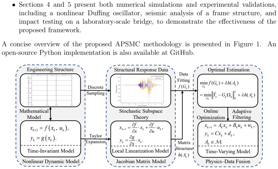
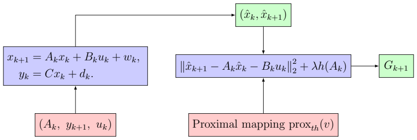
The mechanism is a coupled loop of two classical tools: a Kalman filter that produces the optimal state estimate $\hat{x}_k$ from the current model, and a proximal-gradient step that updates the matrix pair $(A_k, B_k)$ by minimizing $\|\hat{x}_{k+1} - A_k \hat{x}_k - B_k u_k\|^2$ plus a physical regularizer, which is effectively an online least-squares fit against filtered states. What licenses the optimality claim is a stochastic subspace identity: the noise subspace is statistically orthogonal to the signal subspace, so as data grows the residual noise vanishes and the least-squares objective is evaluated against the true Kalman-filtered sequence. Physical priors enter through the proximal mapping, with hard structural constraints such as the block form of a mechanical system's continuous-time matrix acting as projections and soft constraints as regularizers. The upshot is that the time-varying $A_k$ can be read as the Jacobian of the nonlinear dynamics, which gives the identified matrices their physical interpretability.
What would settle it
Run the algorithm on a linear time-invariant system with known $A$, initialize $A_0$ far from the truth with the sensor count below the state dimension, and monitor $\|A_k - A^*\|$: the paper itself reports that in this regime the Kalman filter fails to provide accurate predictions, so the claimed limit $\lim_{i\to\infty}\Delta A_i = 0$ would be violated. A second check targets the constrained version: because the bilinear transform used to impose continuous-time constraints makes that subproblem non-convex, exhibiting two different initial matrices that converge to two different stationary solutions would contradict the global-optimality claim.
Extended reading notes
Core claim
On the paper's own terms, the discovery is that merging stochastic subspace identification with an online proximal-gradient loop turns nonlinear structural estimation into a convex problem with a provable optimum: with infinite data the subspace argument eliminates the noise component, leaving the least-squares target $A^* = \arg\min_A \sum_i \|\hat{x}_{i+1} - A\hat{x}_i\|^2$ built from the true Kalman-filtered states, and each online step solves a convex subproblem of this form, so the paper asserts $\lim_{i\to\infty}\Delta A_i = 0$ and convergence to the theoretically optimal model. Because the system matrix is locally the Jacobian of the dynamics, the identified matrices retain physical meaning, and when structural constraints are imposed through the proximal mapping the method tracks the Jacobian even where purely data-driven fits fail. Experimentally, the claim is that a single 10-second impact-test segment updates the model well enough to predict 19 unseen 10-second tests, with a best normalized mean square error (NMSE) of 0.398%.
Load-bearing premise
The argument assumes that alternating between Kalman filtering, whose state estimates depend on the current system matrix, and a convex least-squares update of that matrix drives the pair to the joint optimum; the paper never proves this coupled fixed-point convergence, and it concedes in Section 5.3 that a poor initial matrix with fewer sensors than states prevents the filter from updating the model correctly.
Editorial extensions
If this is right
- Continuous monitoring becomes a live model-update loop: each new acceleration sample refines the system matrices without storing or reprocessing the full measurement history.
- The identified matrices carry physical meaning, since their block structure approximates the structure's mass, stiffness, and damping, so damage and drift could be read directly from the estimates.
- Extremely short calibration data may suffice: a single 10-second impact-test segment predicted 19 unseen 10-second responses with a minimum NMSE of 0.398%.
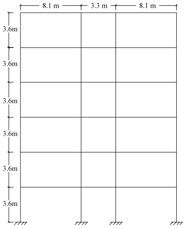
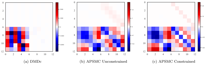
- Physical constraints are what preserve accuracy under noise: on a frame structure with 30% added noise, constrained APSMC held prediction NMSE at 4.35% versus 12.56% for unconstrained APSMC and 34.54% for the global linear baseline.
- The framework extends to arbitrary white-noise distributions and explicit external inputs, covering cases the earlier APSM formulation could not handle.
Reading between the lines
- Because the filter and the matrix update feed each other, a fully rigorous convergence guarantee would require an alternating-minimization or expectation-maximization analysis of the coupled problem; that analysis is not in the paper, and it may impose conditions beyond convexity of each subproblem.
- The paper shows that under weak excitation the least-squares problem is not strictly convex, which suggests a testable extension: characterizing which input spectra let the constrained estimator recover the physical Jacobian rather than merely a minimum-Frobenius-norm fit.
- Nothing in the argument pins the filter to the linear-Gaussian Kalman filter, so the same loop with an unscented or particle filter for non-Gaussian noise is a direct and untested extension.
- Because the proximal step is generic, the loop could in principle be applied to other locally linearizable physical systems, such as identifying contact or friction laws, by changing only the constraint set.
Signed reviews
Editorial analysis
A structured set of objections, weighed in public.
Referee Report
Summary. The paper proposes the Adaptive Physics-Informed System Modeling with Control (APSMC) framework for online identification of time-varying linear state-space models from noisy input–output data. The method alternates between Kalman filtering (or another Bayesian filter) for state estimation and online proximal-gradient updates of the system matrices A and B, subject to physics-based structural constraints. The paper claims a theoretical guarantee, derived from stochastic subspace identification, that as data accumulate the estimates converge to the theoretically optimal solution (Section 3.1), and it validates the method on a Duffing oscillator, a seismic frame response simulation, and impact tests on a scaled bridge model, reporting NMSE values as low as 0.398%. An open-source Python implementation is provided.
Significance. If the central convergence and optimality claims were valid, APSMC would be a notable contribution to online nonlinear structural system identification: it combines state estimation with constrained optimization, provides physically interpretable time-varying system matrices, and is supported by code and by tests in simulation and experiment. The empirical framework is attractive and the reported prediction accuracy on the bridge data is competitive. However, the theoretical guarantee is not established and is contradicted by the paper's own statements; the experimental design involves heavy per-dataset tuning; and one of the interpretability claims rests on an algebraic error. The contribution is therefore currently an interesting heuristic with promising experiments rather than a validated theoretical method.
major comments (4)
- [Sec. 3.1 (Eqs. 24-29), Sec. 5.3, App. B.2] The claimed guarantee lim_{i→∞} ΔA_i = 0 is not proven. The objective (24) is convex for a fixed state sequence, but the regressors x̂_k and targets x̂_{k+1} are outputs of a Kalman filter whose gain and innovation covariance depend on the A being estimated, so the iteration is a coupled stochastic approximation with state-dependent noise. Eq. (26) defines A* as the least-squares fit to the filtered states, so the target is self-referential rather than the data-generating A_true; no contraction, Lyapunov, or stochastic-approximation argument is supplied. The paper's own Sec. 5.3 concedes that with a poor initial A0 the Kalman filter fails and the algorithm cannot update to the correct model, and that it is theoretically unclear whether identity initialization guarantees convergence. Appendix B.2 additionally concedes that the bilinear-transform constraint is non-convex, so proximal gradient does not guarantee a global optimum. These admissions directly contradict the headline guarantee.
- [Sec. 4.1 (Eqs. 46-48)] The equality asserted between the Duffing system and the Jacobian-based time-varying linear system is algebraically false. Substituting J(x) from (46) into (47) yields ẋ₂ = (α - 3βx₁²)x₁ - c x₂ + F cos(ωt) = α x₁ - 3βx₁³ - c x₂ + F cos(ωt), whereas the original system (44) has ẋ₂ = α x₁ - β x₁³ - c x₂ + F cos(ωt); the difference is -2βx₁³. Consequently x_{k+1} = J(x_k) x_k + B_k u_k is not a representation of the nonlinear system, and the numerical agreement of A_k with J(x_k) in Figs. 6-8 is not a valid ground-truth comparison for the claim that A_k tracks the Jacobian.
- [Sec. 5.2 (Table 2)] The experimental evidence does not support the claimed consistent superiority of APSMC. The learning rate t_k is hand-tuned per dataset and varies by four orders of magnitude (0.004 to 100). For sequences 15 and 19, APSMC's NMSE (18.847% and 17.028%) is substantially worse than ERA's (10.065% and 11.164%). The 0.398% figure quoted in the abstract is the minimum over all sensors and datasets, not a typical result. The model order and Hankel dimensions (m = n = 3000) are also determined ad hoc, without sensitivity analysis.
- [Secs. 4-5 (Algorithms 1-2)] The algorithm's reproducibility is compromised by unspecified key hyperparameters. The noise covariances Q, R, and P0 for the Kalman filter, the regularization weight λ in Eq. (37), and the step-size schedule t_k used in the numerical and experimental studies are not reported (except for selected learning rates in Table 2). Without these, the results cannot be replicated, and the claim that the method is 'theoretically optimal' cannot be assessed against the actual implementation.
minor comments (6)
- [Throughout (Figs. 5-22)] Many figures contain extensive text corruption (e.g., strings of '/uni00000013/uni00000018/...'), and numerous figures lack captions; the manuscript must be regenerated cleanly before review.
- [Sec. 2.1, Eq. (2)] Eq. (2) uses squared error E[(x_k - g)^2] for vector states; it should be a vector norm (or sum of squares) to define the MMSE estimator.
- [Sec. 3.2] The statement that noise 'may follow arbitrary distributions of white noise' is an overclaim: Kalman filtering is optimal only under Gaussianity, and the paper neither analyzes nor tests non-Gaussian noise.
- [Sec. 5.3] The analogy between the algorithm and SGD is imprecise: online proximal gradient with sequentially ordered samples is not stochastic gradient descent (which samples randomly), and the convergence properties differ.
- [References] Several key references are unpublished preprints, notably [2] (SSRN) and [31] (arXiv), and results in Secs. 4-5 draw heavily on [31] and [9]; these dependencies should be updated or clarified.
- [Abstract and Sec. 5.2] The abstract's claim of '19 consecutive 10-second time series using only a single initial 10-second segment for model updating' is misleading because Table 2 shows large errors for several sequences and the model was updated sequentially, not held fixed; the description should be precise.
Circularity Check
Section 3.1's convergence-to-optimality claim is self-referential: A* is defined as the least-squares fit to Kalman-filtered states, while the same objective over states produced by the estimated A supplies the 'optimal solution' the algorithm is said to reach.
-
self definitional
[Section 3.1, Eq. (26) and following paragraph (Eqs. 27-29); compare Eq. (24) and Algorithm 1]
"if the true Kalman-filtered state sequence ˆXi were known, the optimal estimate of the system matrix A∗ could be defined as: A∗ = argmin A Pk i=1 ∥ˆxi+1−Aˆxi∥2 2 = ˆYk ˆX† k (26) ... Since the objective function in equation (24) is convex, and each update follows a convex optimization scheme, the algorithm is guaranteed to converge to the global optimum based on the true Kalman-filtered state sequence."
Equation (26) defines the target A* as the least-squares fit to the Kalman-filtered state sequence. Equation (24) (and its APSMC version, Eq. (38)) is the same least-squares objective, but the state matrices Xhat_k and Yhat_k entering it are produced online by a Kalman filter whose gain and state estimates depend on the very A being optimized. Thus the 'global optimum' the algorithm is guaranteed to reach is the minimizer of the algorithm's own, self-referential objective, not an independently specified system matrix. The proof that this minimizer equals A* requires that the online KF state sequence coincide with the 'true Kalman-filtered state sequence' — precisely the fixed-point convergence that is asserted rather than derived.
full rationale
The empirical core of the paper is self-contained: APSMC is benchmarked against DMDc on a frame structure and against ERA/OKID+ERA on a scaled bridge, with predictions evaluated on holdout segments via NMSE. Those comparisons do not reduce to the fitted inputs, and the self-citations to the authors' prior APSM work [2] are not load-bearing for those experiments. The circularity is concentrated in the theoretical optimality claim of Section 3.1. Eq. (26) defines A* as the least-squares fit to a Kalman-filtered state sequence, while the online algorithm (Algorithm 1/2, Eq. (24)/(38)) minimizes the same least-squares objective over state sequences produced by the Kalman filter running with the iteratively updated A. The 'optimal solution' is therefore defined internally as the minimizer of the algorithm's own loss, and the additional claim that this minimizer is the 'true Kalman-filtered state sequence' is a fixed-point assumption that is never proved. The paper's own Section 5.3 concedes that with a poor initial A0 the KF fails and 'it remains theoretically unclear whether initializing A0 as an identity matrix guarantees convergence to the optimal solution,' and Appendix B.2 admits that the bilinear-transform constraints make the optimization non-convex, so proximal gradient does not inherently guarantee global optimality. These admissions confirm that the headline convergence guarantee is an unproved assumption rather than a derived result. Because the target of the theoretical claim is defined by the same objective the algorithm minimizes, the convergence result is partially circular by construction; the numerical and experimental demonstrations retain independent value despite this theoretical gap.
Assumptions & free parameters
free parameters (6)
- Per-test learning rate t_k =
0.004 to 100 (listed per sequence in Table 2)
- Model order n =
50 to 577; n=300 used for the main result
- Hankel matrix dimensions m and n =
m = n = 3000
- Regularization weight λ =
not reported
- Kalman filter noise covariances Q, R, P0 =
not reported
- Iteration count =
100 to 1100 iterations
assumptions (5)
- domain assumption The true system is well approximated by a linear time-varying state-space model with zero-mean white process and measurement noise.
- domain assumption The Kalman filter provides the minimum-mean-square-error state estimate for the evolving model at each step.
- standard math The signal and noise subspaces in stochastic subspace identification are asymptotically orthogonal, so the projection in Eq. (13) removes all noise as j→∞.
- ad hoc to paper The objective in Eq. (24) is convex at each update, so the proximal gradient step converges to its global minimum.
- domain assumption The physical constraint structure (e.g., Jacobian form [0 1; Unknown -0.1] or symmetric lower blocks) is known a priori.
Cite this review
Pith. "Pith review of Adaptive Physics-Informed System Modeling with Control for Nonlinear Structural System Estimation." pith.science (2026). https://pith.science/paper/7EM4H6WY
@misc{pith2026250506525,
  author       = {Pith},
  title        = {Pith review of: Adaptive Physics-Informed System Modeling with Control for Nonlinear Structural System Estimation},
  year         = {2026},
  howpublished = {\url{https://pith.science/paper/7EM4H6WY}},
  note         = {Machine review of arXiv:2505.06525}
}
read the original abstract
Accurately capturing the nonlinear dynamic behavior of structures remains a significant challenge in mechanics and engineering. Traditional physics-based models and data-driven approaches often struggle to simultaneously ensure model interpretability, noise robustness, and estimation optimality. To address this issue, this paper proposes an Adaptive Physics-Informed System Modeling with Control (APSMC) framework. By integrating Kalman filter-based state estimation with physics-constrained proximal gradient optimization, the framework adaptively updates time-varying state-space model parameters while processing real-time input-output data under white noise disturbances. Theoretically, this process is equivalent to real-time tracking of the Jacobian matrix of a nonlinear dynamical system. Within this framework, we leverage the theoretical foundation of stochastic subspace identification to demonstrate that, as observational data accumulates, the APSMC algorithm yields state-space model estimates that converge to the theoretically optimal solution. The effectiveness of the proposed framework is validated through numerical simulations of a Duffing oscillator and the seismic response of a frame structure, as well as experimental tests on a scaled bridge model. Experimental results show that, under noisy conditions, APSMC successfully predicts 19 consecutive 10-second time series using only a single initial 10-second segment for model updating, achieving a minimum normalized mean square error (NMSE) of 0.398%. These findings demonstrate that the APSMC framework not only offers superior online identification and denoising performance but also provides a reliable foundation for downstream applications such as structural health monitoring, real-time control, adaptive filtering, and system identification.
Figures


Figures from the paper (19 more)








Reference graph
Works this paper leans on
-
[1]
B. Herrmann, P. J. Baddoo, R. Semaan, S. L. Brunton, B. J. McKeon, Data-driven resolvent analysis 918 A10. doi:10.1017/jfm.2021.337. URL https://www.cambridge.org/core/product/identifier/ S0022112021003372/type/journal_article
-
[2]
B. Chen, Y. Wang, J. Yang, J. Ou, Adaptive physics-informed system modeling for online structural dynamic simulation, Available at SSRN 5097818
-
[3]
J. L. Proctor, P. A. Eckhoff, Discovering dynamic patterns from infectious disease data using dynamic mode decomposition, International health 7 (2) (2015) 139–145
2015
-
[4]
H. K. Khalil, J. W. Grizzle, Nonlinear systems, Vol. 3, Prentice hall Upper Saddle River, NJ, 2002
work page 2002
-
[5]
Meirovitch, Computational methods in structural dynamics, Vol
L. Meirovitch, Computational methods in structural dynamics, Vol. 5, Springer Science & Business Media, 1980
work page 1980
-
[6]
J. H. Ferziger, M. Peri´ c, R. L. Street, Computational methods for fluid dynamics, springer, 2019
work page 2019
- [7]
-
[8]
H. Zhang, C. W. Rowley, E. A. Deem, L. N. Cattafesta, Online dynamic mode decom- position for time-varying systems 18 (3) 1586–1609. doi:10.1137/18M1192329. URL https://epubs.siam.org/doi/10.1137/18M1192329
Show all 60 references
-
[9]
B. Chen, Y. Wang, Minimal realization time-delay koopman analysis for nonlinear sys- tem identification (2025)
2025
-
[10]
B. Chen, Y. Wang, Online physics-informed dynamic mode decomposition: Theory and applications, arXiv preprint arXiv:2412.03609 (2024)
2024 arXiv
-
[11]
Kirchdoerfer, M
T. Kirchdoerfer, M. Ortiz, Data-driven computational mechanics, Computer Methods in Applied Mechanics and Engineering 304 (2016) 81–101
2016
-
[12]
De Lorenzis, Automated discovery of hyperelastic material models, Constitutive Mod- els for Rubbers XIII (2025) 3–13
L. De Lorenzis, Automated discovery of hyperelastic material models, Constitutive Mod- els for Rubbers XIII (2025) 3–13
2025
-
[13]
Mezi´ c, Analysis of fluid flows via spectral properties of the koopman operator 45 (1) 357–378
I. Mezi´ c, Analysis of fluid flows via spectral properties of the koopman operator 45 (1) 357–378. doi:10.1146/annurev-fluid-011212-140652 . URL https://www.annualreviews.org/doi/10.1146/ annurev-fluid-011212-140652
-
[14]
S. L. Brunton, M. Budiˇ si´ c, E. Kaiser, J. N. Kutz, Modern koopman theory for dynamical systems. arXiv:2102.12086. URL http://arxiv.org/abs/2102.12086
-
[15]
Mezi´ c, Spectral properties of dynamical systems, model reduction and decompositions, Nonlinear Dynamics 41 (2005) 309–325
I. Mezi´ c, Spectral properties of dynamical systems, model reduction and decompositions, Nonlinear Dynamics 41 (2005) 309–325
2005
-
[16]
B. O. Koopman, Hamiltonian systems and transformation in hilbert space, Proceedings of the National Academy of Sciences 17 (5) (1931) 315–318
1931
-
[17]
B. O. Koopman, J. v. Neumann, Dynamical systems of continuous spectra, Proceedings of the National Academy of Sciences 18 (3) (1932) 255–263
1932
-
[18]
J. H. Tu, C. W. Rowley, D. M. Luchtenburg, S. L. Brunton, J. N. Kutz, On dynamic mode decomposition: Theory and applications 1 (2) 391–421. arXiv:1312.0041, doi: 10.3934/jcd.2014.1.391. URL http://arxiv.org/abs/1312.0041
2014 arXiv
-
[19]
P. J. Schmid, Dynamic mode decomposition of numerical and experimental data 656 5–28. doi:10.1017/S0022112010001217. URL https://www.cambridge.org/core/product/identifier/ S0022112010001217/type/journal_article
-
[20]
P. J. Schmid, Dynamic mode decomposition and its variants 54 (1) 225–254. doi:10.1146/annurev-fluid-030121-015835 . URL https://www.annualreviews.org/doi/10.1146/ annurev-fluid-030121-015835 35
-
[21]
M. O. Williams, I. G. Kevrekidis, C. W. Rowley, A data–driven approximation of the koopman operator: Extending dynamic mode decomposition, Journal of Nonlinear Sci- ence 25 (2015) 1307–1346
2015
-
[22]
Yeung, S
E. Yeung, S. Kundu, N. Hodas, Learning deep neural network representations for koop- man operators of nonlinear dynamical systems. arXiv:1708.06850. URL http://arxiv.org/abs/1708.06850
-
[23]
J. Wu, M. Luo, D. Xiao, C. C. Pain, B. C. Khoo, Koopman dynamic-oriented deep learn- ing for invariant subspace identification and full-state prediction of complex systems, Computer Methods in Applied Mechanics and Engineering 429 (2024) 117071
2024
-
[24]
S. L. Brunton, J. L. Proctor, J. N. Kutz, Discovering governing equations from data by sparse identification of nonlinear dynamical systems, Proceedings of the national academy of sciences 113 (15) (2016) 3932–3937
2016
-
[25]
Rosafalco, P
L. Rosafalco, P. Conti, A. Manzoni, S. Mariani, A. Frangi, Ekf–sindy: Empowering the extended kalman filter with sparse identification of nonlinear dynamics, Computer Methods in Applied Mechanics and Engineering 431 (2024) 117264
2024
-
[26]
J. M. Brownjohn, Structural health monitoring of civil infrastructure, Philosophical Transactions of the Royal Society A: Mathematical, Physical and Engineering Sciences 365 (1851) (2007) 589–622
2007
-
[27]
P. J. Baddoo, B. Herrmann, B. J. McKeon, J. N. Kutz, S. L. Brunton, Physics-informed dynamic mode decomposition (pidmd). arXiv:2112.04307. URL http://arxiv.org/abs/2112.04307
-
[28]
G. E. Karniadakis, I. G. Kevrekidis, L. Lu, P. Perdikaris, S. Wang, L. Yang, Physics- informed machine learning, Nature Reviews Physics 3 (6) (2021) 422–440
2021
-
[29]
Peeters, G
B. Peeters, G. D. Roeck, Reference-based stochastic subspace identification for output- only modal analysis
-
[30]
E. A. Wan, R. Van Der Merwe, The unscented kalman filter for nonlinear estimation, in: Proceedings of the IEEE 2000 adaptive systems for signal processing, communications, and control symposium (Cat. No. 00EX373), Ieee, 2000, pp. 153–158
2000
-
[31]
B. Chen, J. Zhang, Y. Wang, Principal component stochastic subspace identification for output-only modal analysis, arXiv preprint arXiv:2504.00317 (2025)
2025 arXiv
-
[32]
Juang, R
J.-N. Juang, R. S. Pappa, An eigensystem realization algorithm for modal parameter identification and model reduction, Journal of guidance, control, and dynamics 8 (5) (1985) 620–627
1985
-
[33]
Van Overschee, B
P. Van Overschee, B. De Moor, Subspace identification for linear systems: The- ory—Implementation—Applications, Springer Science & Business Media, 2012. 36
2012
-
[34]
Viberg, Subspace-based methods for the identification of linear time-invariant sys- tems, Automatica 31 (12) (1995) 1835–1851
M. Viberg, Subspace-based methods for the identification of linear time-invariant sys- tems, Automatica 31 (12) (1995) 1835–1851
1995
-
[35]
W. Wen, C. Zhang, C. Zhai, Rapid seismic response prediction of rc frames based on deep learning and limited building information, Engineering Structures 267 (2022) 114638
2022
-
[36]
J. W. Baker, C. A. Cornell, Pacific earthquake engineering research center, University of California, Berkeley (2006)
2006
-
[37]
Chopra, Dynamics of structures: Theory and applications to earthquake engineering 4th edition prentice hall englewood cliffs (2011)
A. Chopra, Dynamics of structures: Theory and applications to earthquake engineering 4th edition prentice hall englewood cliffs (2011)
2011
-
[38]
J. L. Proctor, S. L. Brunton, J. N. Kutz, Dynamic mode decomposition with control 15 (1) 142–161. doi:10.1137/15M1013857. URL http://epubs.siam.org/doi/10.1137/15M1013857
-
[39]
Juang, M
J.-N. Juang, M. Phan, L. G. Horta, R. W. Longman, Identification of observer/kalman filter markov parameters: Theory and experiments
-
[40]
S. Pan, K. Duraisamy, On the structure of time-delay embedding in linear models of non-linear dynamical systems 30 (7) 073135. doi:10.1063/5.0010886. URL https://pubs.aip.org/cha/article/30/7/073135/321507/ On-the-structure-of-time-delay-embedding-in-linear
-
[41]
S. L. Brunton, Chaos as an intermittently forced linear system
-
[42]
Arbabi, I
H. Arbabi, I. Mezi´ c, Ergodic theory, dynamic mode decomposition and computation of spectral properties of the koopman operator. arXiv:1611.06664, doi:10.1137/ 17M1125236. URL http://arxiv.org/abs/1611.06664
-
[43]
Gavish, D
M. Gavish, D. L. Donoho, The optimal hard threshold for singular values is 4/ √ 3, IEEE Transactions on Information Theory 60 (8) (2014) 5040–5053
2014
-
[44]
E. J. Candes, X. Li, Y. Ma, J. Wright, Robust principal component analysis? arXiv: 0912.3599. URL http://arxiv.org/abs/0912.3599
-
[45]
P. L. Combettes, V. R. Wajs, Signal recovery by proximal forward-backward splitting, Multiscale modeling & simulation 4 (4) (2005) 1168–1200
2005
-
[46]
Schmidt, N
M. Schmidt, N. Roux, F. Bach, Convergence rates of inexact proximal-gradient methods for convex optimization, Advances in neural information processing systems 24 (2011)
2011
-
[47]
Suzuki, Dual averaging and proximal gradient descent for online alternating direction multiplier method, in: International Conference on Machine Learning, PMLR, 2013, pp
T. Suzuki, Dual averaging and proximal gradient descent for online alternating direction multiplier method, in: International Conference on Machine Learning, PMLR, 2013, pp. 392–400. 37
2013
-
[48]
Johnson, T
R. Johnson, T. Zhang, Accelerating stochastic gradient descent using predictive variance reduction, Advances in neural information processing systems 26 (2013)
2013
-
[49]
Schmidt, N
M. Schmidt, N. Le Roux, F. Bach, Minimizing finite sums with the stochastic average gradient, Mathematical Programming 162 (2017) 83–112
2017
-
[50]
Defazio, F
A. Defazio, F. Bach, S. Lacoste-Julien, Saga: A fast incremental gradient method with support for non-strongly convex composite objectives, Advances in neural information processing systems 27 (2014)
2014
-
[51]
Nitanda, Stochastic proximal gradient descent with acceleration techniques, Ad- vances in neural information processing systems 27 (2014)
A. Nitanda, Stochastic proximal gradient descent with acceleration techniques, Ad- vances in neural information processing systems 27 (2014)
2014
-
[52]
C. Jin, P. Netrapalli, M. I. Jordan, Accelerated gradient descent escapes saddle points faster than gradient descent, in: Conference On Learning Theory, PMLR, 2018, pp. 1042–1085
2018
-
[53]
Qian, On the momentum term in gradient descent learning algorithms, Neural net- works 12 (1) (1999) 145–151
N. Qian, On the momentum term in gradient descent learning algorithms, Neural net- works 12 (1) (1999) 145–151
1999
-
[54]
W. Liu, L. Chen, Y. Chen, W. Zhang, Accelerating federated learning via momentum gradient descent, IEEE Transactions on Parallel and Distributed Systems 31 (8) (2020) 1754–1766
2020
-
[55]
R. Ward, X. Wu, L. Bottou, Adagrad stepsizes: Sharp convergence over nonconvex landscapes, Journal of Machine Learning Research 21 (219) (2020) 1–30
2020
-
[56]
Duchi, E
J. Duchi, E. Hazan, Y. Singer, Adaptive subgradient methods for online learning and stochastic optimization., Journal of machine learning research 12 (7) (2011)
2011
-
[57]
D. P. Kingma, J. Ba, Adam: A method for stochastic optimization, arXiv preprint arXiv:1412.6980 (2014)
2014 arXiv
-
[58]
F. Zou, L. Shen, Z. Jie, W. Zhang, W. Liu, A sufficient condition for convergences of adam and rmsprop, in: Proceedings of the IEEE/CVF Conference on computer vision and pattern recognition, 2019, pp. 11127–11135
2019
-
[59]
P. L. Combettes, J.-C. Pesquet, Proximal splitting methods in signal processing, Fixed- point algorithms for inverse problems in science and engineering (2011) 185–212
2011
-
[60]
P. J. Baddoo, B. Herrmann, B. J. McKeon, J. Nathan Kutz, S. L. Brunton, Physics- informed dynamic mode decomposition 479 (2271) 20220576.doi:10.1098/rspa.2022. 0576. URL https://royalsocietypublishing.org/doi/10.1098/rspa.2022.0576 38
2022
Reviewed August 15, 2026 · model on record in the stance chip above.
Discussion (0). Continue with ORCID to comment.