REVIEW 4 major objections 5 minor 42 references
The classification of real and bogus transients using active learning and semi-supervised learning
T0 review · 4 major / 5 minor · reviewed 2026-08-11 · deepseek-v4-flash
Pith's one-line read A real/bogus transient classifier built from only 1000 labels can match fully supervised models trained on 2500.
desk verdict Solid, honest AL+SSL real/bogus paper whose accuracy claims are limited by knowingly non-representative labels; deserves review but not the deployment framing. read the letter →
The pith
A machine-rendered reading of the paper's core claim, the machinery that carries it, and where it could break.
The reading
What carries the argument
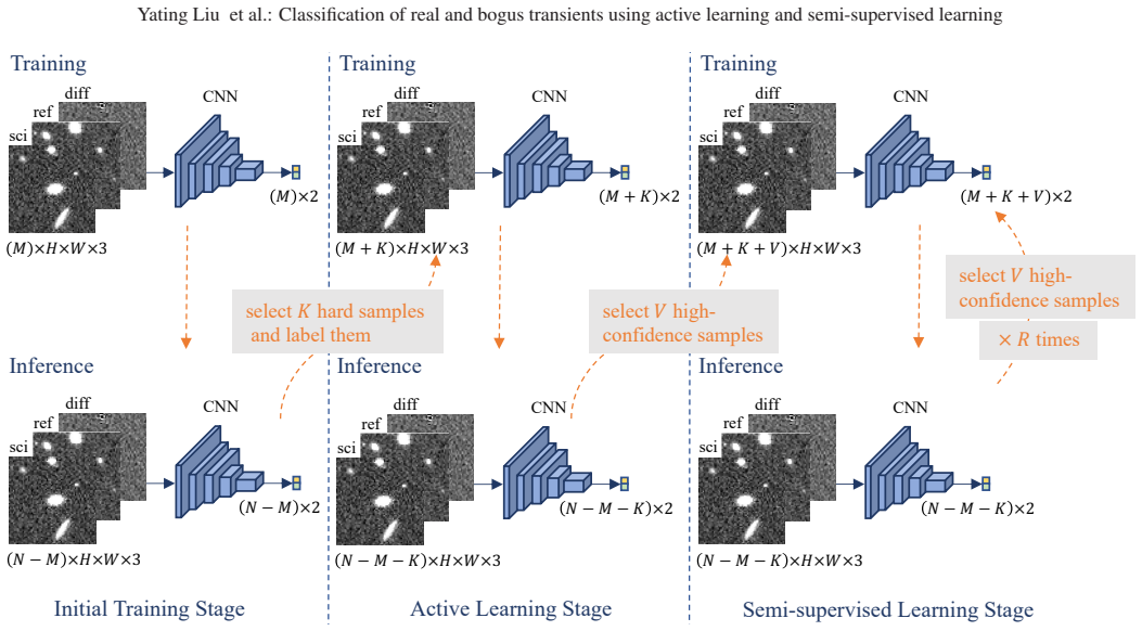
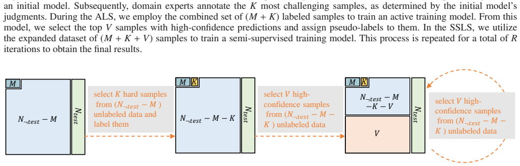
The central mechanism is the three-stage RB-C1000 pipeline built on a ResNet-18 backbone taking three input channels (science, reference, and difference image stamps of 63x63 pixels). The initial training stage (ITS) trains on M=900 labeled samples and ranks unlabeled data by prediction confidence to identify the K=100 hardest samples. The active learning stage (ALS) retrains on the labeled set of 1000 samples and selects V pseudo-labeled samples whose confidence exceeds a threshold of τ=0.95. The semi-supervised learning stage (SSLS) retrains from scratch on labeled plus pseudo-labeled data and repeats R=3 times. This combination lets the model exploit both expert-selected hard examples and abundant unlabeled data without extra human annotation.
What would settle it
Take a fresh sample of alert streams from a running survey, label every candidate by expert visual inspection (including non-supernova real sources such as AGN variability and moving objects), and run the RB-C1000 model trained on the paper's recipe; if accuracy on this expert-labeled test set falls well below 98% or the false-negative rate on non-supernova real sources is much higher than the reported ~1.8%, the claimed generalization does not hold.
Extended reading notes
Core claim
The paper's central claim is that a real/bogus classifier built with only 1000 labeled samples can perform as well as a fully supervised model trained on thousands of random labels. In the RB-C1000 pipeline the initial supervised model selects the K=100 hardest unlabeled samples for expert annotation; the active model then picks V high-confidence samples and assigns them pseudo-labels; and the semi-supervised model retrains on the expanded set for R=3 iterations. On the ZTF-NEWg, ZTF-NEWr, and ZTF-NEWm datasets this yields average accuracies of 98.8%, 98.8%, and 98.6%, with the mixed-band ZTF-NEWm result (98.6%) exceeding the fully supervised ResNet-18 baseline trained on 2500 random labels (98.4%). The authors frame this as a practical route to deploying deep-learning real/bogus classification at the start of a survey, when annotation resources are limited.
Load-bearing premise
The results depend on the labels being trustworthy: real sources are only supernovae reported to TNS, and the bogus set is a random sample of detection candidates that the authors say may contain a few real detections, so label contamination would inflate the measured accuracy.
Editorial extensions
If this is right
- Surveys like WFST and LSST can deploy a deep-learning real/bogus filter early in operations with only about 1000 human labels, reducing annotation cost and enabling rapid follow-up.
- The RB-C1000 recipe improves over random labeling by 1.4-7.2 percentage points in summed performance and over labeled-only training by 4.1-8.7 points, depending on the band.
- A fully supervised model needs roughly 2500 random labels to match RB-C1000's 1000-label performance on the mixed-band dataset, so the method is more label-efficient.
- The pseudo-labeling iterations saturate around R=3, and using 5000-10000 unlabeled samples balances performance and training time.
- The classifier is intended to be integrated into the WFST data processing pipeline for early-survey transient classification.
Reading between the lines
- The same two-stage annotation strategy (label hardest, then pseudo-label confident rest) could be transferred to other label-scarce astronomical classification problems such as anomaly detection or supernova typing, where the gains from active selection on harder data appear largest.
- Because the mixed-band dataset showed the largest active-learning gain, the method is likely most valuable when the data distribution is heterogeneous; a direct test would be to run RB-C1000 on multi-band or multi-telescope inputs with different noise properties.
- The reported band asymmetry (r-to-g transfer fails while g-to-r works) implies that a single cross-band model is not safe; an inference is that WFST could train per-band RB-C1000 models using 1000 labels each, which the pipeline's cost makes feasible.
- If the pseudo-label threshold or iteration count is tuned on one telescope's stamps, the optimal values may shift for another telescope; a testable extension is to re-scan τ and R on LSST-like simulated stamps.
Editorial analysis
A structured set of objections, weighed in public.
Referee Report
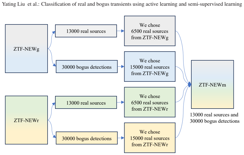
Summary. The paper proposes RB-C1000, a deep-learning pipeline for real/bogus transient classification that combines active learning with pseudo-labeling-based semi-supervised learning. The method starts from M=900 labeled samples, has experts label K=100 hard samples, then iteratively pseudo-labels V high-confidence unlabeled samples over R rounds. Using three newly compiled ZTF datasets (ZTF-NEWg, ZTF-NEWr, ZTF-NEWm), each with 13,000 real sources (TNS supernovae) and 30,000 unvetted bogus candidates, the authors report mean accuracies of 98.8%, 98.8%, and 98.6% with only 1,000 labels, and argue that this surpasses a fully supervised ResNet-18 trained on 2,500 random labels. The paper includes repeated experiments (five trials), confidence intervals on metrics, and publicly available code and data. The authors repeatedly and explicitly caution that the datasets are not representative of the general alert stream.
Significance. If the reported efficiency gain is real, the method is a useful contribution to time-domain astronomy: it would allow early-survey operations to build a competitive classifier with far fewer manual labels. The algorithmic pipeline is coherent, the experiments are repeated five times with reported standard deviations, and the code and datasets are public, which are strengths. The central limitation is that the constructed labels do not match the stated deployment target: real is defined as TNS-reported supernovae, while bogus is a random, unvetted sample of detection candidates possibly containing real astrophysical sources. The paper acknowledges this in Section 2 and again in Sections 4 and 5, but the abstract and conclusion nevertheless frame the results as enabling general real-source discovery in WFST. The method's internal comparisons (active learning vs. random selection, SSL vs. no SSL) are meaningful on the constructed datasets, but the absolute performance and the headline efficiency claim require either representative labels or a considerably more cautious interpretation.
major comments (4)
- [Section 2, Section 5] The label definitions undermine the central deployment claim. Real sources are only TNS supernovae from 2019–2022, and bogus sources are randomly drawn detection candidates that, as the text acknowledges, 'might contain a few real detections.' The reported 98.8%/98.8%/98.6% accuracies therefore measure separation between TNS supernovae and unvetted artifacts, not performance on the general alert stream (stellar flares, AGN variability, faint SNe, moving objects, etc.). The paper already states this caveat, but the abstract and conclusion still claim the method can 'discover real sources that vary in brightness over time in the early stage of WFST.' Please either provide a validation set with representative, vetted real and bogus labels (e.g., a human-vetted alert sample or a set including known non-SN real sources), or explicitly restrict the performance claims to 'SNe-like real sources' and remove the implication of general WFST readiness.
- [Section 4.3, Table A.3, Table A.4, Table A.5] Several hyperparameters were selected using the same test sets on which final performance is reported. The text states that R=3 was chosen because it 'often shows the best performance on the overall indicator on these three datasets'; Table A.3 selects 10,000 unlabeled samples partly from test-set performance; Table A.4 selects M/K ratio 0.9 based on the highest sum on ZTF-NEWm. This makes the reported numbers optimistic and the efficiency comparison in Table A.6 circular in the sense that the configuration was tuned on the same test set. Please use a separate validation split for hyperparameter selection and report test-set results only for the selected configuration, or present the full set of configurations with an appropriate correction for multiple comparisons.
- [Table A.6, Section 4.3] The headline efficiency claim is not statistically established. RB-C1000 (ZTF-NEWm, sum = 587.5 ± 0.8) is compared with a fully supervised model using 2,500 random labels (sum = 586.3 ± 2.0). The difference in means is 1.2 points; using the reported standard deviations and five repeats, the difference is within approximately 1.3 standard errors, i.e., not significant at the usual 0.05 level. Please report a paired comparison across the five repeats (e.g., paired t-test or Wilcoxon signed-rank test) or otherwise quantify the uncertainty of the improvement, and adjust the claim 'significantly higher efficiency' accordingly.
- [Section 4.3, Table A.2] The active-learning component's standalone benefit is not consistently demonstrated. On ZTF-NEWr, adding the K hard samples degrades the ALS result relative to ITS (sum 581.4 vs. 581.7), and the final gain appears only after semi-supervised learning. The current separate attribution of '1.4%, 3.4%, and 7.2%' to active learning and '4.1%, 8.7%, and 7.3%' to semi-supervised learning is a post-hoc decomposition of a pipeline with interacting components. Please present an ablation that isolates each component's marginal contribution under the same hyperparameter selection procedure, or interpret the gains as joint effects.
minor comments (5)
- [Section 5] In the concluding paragraph, 'newly complied datasets' should be 'newly compiled datasets.'
- [Figure 6] The figure labels contain 'T rainingCNN' and 'InferenceCNN' with irregular spacing; please clean up the figure text.
- [Section 4.1] The validation set is taken from the (M+K) labeled samples rather than from a separate pool; this is acceptable for model selection but should be stated more explicitly, since it means the 'validation' performance is not an unbiased estimate of generalization to the unlabeled pool.
- [Section 2] The bogus sample construction uses only fields 774–780 on a single date (January 2, 2021). The paper should note whether any real sources from those fields on that date were excluded from the bogus pool, and how the random selection avoids overlap with the real-source set from the same fields.
- [Table A.1] The 'overall performance' metric (sum of six indicators) is not a standard evaluation measure and mixes quantities with different scales; consider reporting it as a secondary diagnostic or justifying its use.
Circularity Check
The reported 98.8/98.8/98.6 accuracies are maxima over hyperparameters (R, unlabeled-pool size, M/K ratio) selected on the same test set used for evaluation, so the headline numbers are partly fitted rather than independent held-out predictions.
-
fitted input called prediction
[Section 4.3, 'Effect of the count of unlabeled data usage', 'Effect of stability on different selections of M and K', and Table A.1/A.3/A.4]
"We notice that SSLS ( R = 3) often shows the best performance on the overall indicator on these three datasets we collected, so we set R = 3 in this paper and the remaining experiments ... are all based on the condition R = 3. ... It can be seen from experiments that 10000 unlabeled sample usage size often give the best results. ... All other experimental results ... were obtained using the case of 10000 unlabeled data usage. ... The highest overall performance is achieved at ratios of 0.9, resulting in performances of 587.5%."
The headline accuracies (98.8%, 98.8%, 98.6%) are computed on the same 10% test split that was used to choose R=3, the 10000-sample unlabeled pool, and the M:K=900:100 ratio. The paper explicitly selects each configuration as the one giving the best or near-best overall performance on the three evaluation datasets, then reports the resulting test-set accuracy as the method's result. Thus the reported metric is, by construction, a maximum over the test set rather than an unbiased prediction for an independent test set. The efficiency comparison against the fully supervised model in Table A.6 inherits these test-selected settings, so the claimed gain of using only 1000 labels is partly a fitted selection effect rather than a standalone prediction of the method.
full rationale
The paper is otherwise empirically self-contained: it builds three new ZTF datasets, trains the RB-C1000 pipeline with 1000 labels, and measures accuracy on held-out test samples; there is no load-bearing self-citation chain and no uniqueness theorem smuggled in. The dataset-construction limitation in Section 2, namely that 'real' sources are only TNS-reported supernovae and that the randomly drawn bogus candidates 'might contain a few real detections,' is a real external-validity caveat, but it is not circularity because the reported metrics are measured against those same constructed labels and the authors explicitly warn that performance may not transfer to the general alert stream. The principal circularity concern is the test-set-based selection of R, unlabeled-pool size, and the M/K ratio; picking the configuration with the best test performance and then presenting that test performance as the method's result makes the headline accuracies partially fitted choices rather than independent predictions. This warrants a score of 6 under the fitted-input-called-prediction pattern, while noting that the active-learning and semi-supervised-learning components still have independent algorithmic content.
Assumptions & free parameters
free parameters (5)
- M (initial labeled sample count) =
900
- K (hard samples labeled by experts) =
100
- tau (confidence threshold) =
0.95
- R (SSLS retraining rounds) =
3
- Unlabeled data pool size =
10000
assumptions (4)
- domain assumption Pseudo-labels above tau=0.95 are accurate enough to train on.
- domain assumption The ZTF datasets are a sufficient proxy for WFST/LSST alert streams.
- domain assumption 63x63 triplet stamps with 1.012 arcsec/pixel encode the needed information.
- standard math ResNet-18 is a suitable backbone.
Cite this review
Pith. "Pith review of The classification of real and bogus transients using active learning and semi-supervised learning." pith.science (2026). https://pith.science/paper/7F7CCVSD
@misc{pith2026241202409,
  author       = {Pith},
  title        = {Pith review of: The classification of real and bogus transients using active learning and semi-supervised learning},
  year         = {2026},
  howpublished = {\url{https://pith.science/paper/7F7CCVSD}},
  note         = {Machine review of arXiv:2412.02409}
}
read the original abstract
Deep-learning-based methods have been favored in astrophysics owing to their adaptability and remarkable performance and have been applied to the task of the classification of real and bogus transients. Different from most existing approaches which necessitate massive yet expensive annotated data, We aim to leverage training samples with only 1000 labels available to discover real sources that vary in brightness over time in the early stage of the WFST 6-year survey. Methods. We present a novel deep-learning method that combines active learning and semi-supervised learning to construct a competitive real/bogus classifier. Our method incorporates an active learning stage, where we actively select the most informative or uncertain samples for annotation. This stage aims to achieve higher model performance by leveraging fewer labeled samples, thus reducing annotation costs and improving the overall learning process efficiency. Furthermore, our approach involves a semi-supervised learning stage that exploits the unlabeled data to enhance the model's performance and achieve superior results compared to using only the limited labeled data.
Figures


Figures from the paper (7 more)




Reference graph
Works this paper leans on
-
[1]
Abell, P. A., Allison, J., Anderson, S. F., et al. 2009, arXiv preprint arXiv:0912.0201 https://arxiv.org/abs/0912.0201
arXiv 2009
-
[2]
Acero-Cuellar, T., Bianco, F., Dobler, G., et al. 2022, AJ, 166, 115 https://arxiv.org/abs/2203.07390
work page Pith review arXiv 2022
-
[3]
Identifying Transients in the Dark Energy Survey using Convolutional Neural Networks
Ayyar, V., Knop Jr, R., Awbrey, A., et al. 2022, astro-ph.IM arXiv:2203.09908 https://arxiv.org/abs/2203.09908
work page Pith review arXiv 2022
-
[4]
How to Find More Supernovae with Less Work: Object Classification Techniques for Difference Imaging
Bailey, S., Aragon, C., Romano, R., et al. 2007, AJ, 665, 1246 https://arxiv.org/abs/0705.0493
work page Pith review arXiv 2007
-
[5]
Bellm, E. C., Kulkarni, S. R., Graham, M. J., et al. 2018, Publ. Astron. Soc. Pac., 131, 018002 https://arxiv.org/abs/1902.01932
arXiv 2018
-
[6]
Bennett, K., & Demiriz, A. 1998, NeurIPS, 11 https://proceedings.neurips.cc/paper/1998/hash/b710915795b9e9c02cf10d6d2bdb688c-Abstract.html
work page 1998
-
[7]
Bertin, E., & Arnouts, S. 1996, ASTROPHYS J SUPPL S, 117, 393 https://aas.aanda.org/articles/aas/abs/1996/08/ds1060/ds1060.html
work page 1996
-
[8]
2010, Astrophysics Source Code Library, ascl-1010
Bertin, E. 2010, Astrophysics Source Code Library, ascl-1010. https://www.astromatic.net/software/swarp/
work page 2010
Show all 42 references
-
[9]
W., Poznanski, D., et al
Brink, H., Richards, J. W., Poznanski, D., et al. 2013, MNRAS, 435, 1047 https://arxiv.org/abs/1209.3775
2013 arXiv
- [10]
-
[12]
C., Magnier, E
Chambers, K. C., Magnier, E. A., Metcalfe, N., et al. 2016, arXiv preprint arXiv:1612.05560 https://arxiv.org/abs/1612.05560
2016 arXiv
-
[13]
2009, IEEE trans
Chapelle, O., Scholkopf, B., & Zien, A. 2009, IEEE trans. neural netw., 20, 542 https://doi.org/10.1109/TNN.2009.2015974
2009
-
[14]
Dark Energy Survey Collaboration, 2005, Int J Mod Phys A, 20, 3121 https://arxiv.org/abs/astro-ph/0510346
2005 arXiv
-
[15]
A., Mahabal, A., Masci, F
Duev, D. A., Mahabal, A., Masci, F. J., et al. 2019, MNRAS, 489, 3582 https://doi.org/10.1093/mnras/stz2357
2019 doi
-
[16]
C., San Martín, J., et al
Förster, F., Maureira, J. C., San Martín, J., et al. 2016, AJ, 832, 155 https://arxiv.org/abs/1609.03567
2016 arXiv
-
[17]
A., D’Andrea, C
Goldstein, D. A., D’Andrea, C. B., Fischer, J. A., et al. 2015, AJ, 150, 82 https://arxiv.org/abs/1504.02936
2015 arXiv
-
[18]
2017, MNRAS, 499, 3130 https://arxiv.org/abs/2004.13877
Gómez, C., Neira, M., Hernández Hoyos, M., et al. 2017, MNRAS, 499, 3130 https://arxiv.org/abs/2004.13877
2017 arXiv
-
[19]
2022, MNRAS, 513, 1742 https://doi.org/10.1093/mnras/stac983
Goode, S., Cooke, J., Zhang, J., et al. 2022, MNRAS, 513, 1742 https://doi.org/10.1093/mnras/stac983
2022 doi
-
[20]
2017, ICCV, 2961 https://arxiv.org/abs/1703.06870
He, K., Gkioxari, G., Dollár, P., et al. 2017, ICCV, 2961 https://arxiv.org/abs/1703.06870
2017 arXiv
-
[21]
2016, CVPR, 770 https://arxiv.org/abs/1512.03385
He, K., Zhang, X., Ren, S. 2016, CVPR, 770 https://arxiv.org/abs/1512.03385
2016 arXiv
-
[22]
2021, EXP ASTRON, 51, 319 https://arxiv.org/abs/2104.13950
Hosenie, Z., Bloemen, S., Groot, P., et al. 2021, EXP ASTRON, 51, 319 https://arxiv.org/abs/2104.13950
2021 arXiv
-
[23]
2022, Universe, 9, 7 https://arxiv.org/abs/2212.11535
Hu, M., Hu, L., Jiang, J., et al. 2022, Universe, 9, 7 https://arxiv.org/abs/2212.11535
2022 arXiv
-
[24]
1999, ICML, 99, 200 https://proceedings.neurips.cc/paper/1998/hash/b710915795b9e9c02cf10d6d2bdb688c-Abstract.html
Joachims, T. 1999, ICML, 99, 200 https://proceedings.neurips.cc/paper/1998/hash/b710915795b9e9c02cf10d6d2bdb688c-Abstract.html
1999
-
[25]
L., Lyman, J., Steeghs, D., et al
Killestein, T. L., Lyman, J., Steeghs, D., et al. 2021, MNRAS, 503, 4838 https://arxiv.org/abs/2102.09892
2021 arXiv
-
[26]
LeCun, Y., Boser, B., Denker, J. S. 1989, Neural Comput, 1, 541 https://doi.org/10.1162/neco.1989.1.4.541
1989 doi
-
[27]
2022, A&A 664, A81 https://arxiv.org/abs/2112.10280
Makhlouf, K., Turpin, D., Corre, D., et al. 2022, A&A 664, A81 https://arxiv.org/abs/2112.10280
2022 arXiv
-
[28]
2016, PASJ, psw096 https://doi.org/10.1093/pasj/psw096
Morii, M., Ikeda, S., Tominaga, N., et al. 2016, PASJ, psw096 https://doi.org/10.1093/pasj/psw096
2016 doi
-
[29]
2017, Automatic differentiation in pytorch https://openreview.net/forum?id=BJJsrmfCZ
Paszke, A., Gross, S., Chintala, S., et al. 2017, Automatic differentiation in pytorch https://openreview.net/forum?id=BJJsrmfCZ
2017
-
[30]
Prince, M. 2004, J. Eng. Educ., 93, 223 https://onlinelibrary.wiley.com/doi/abs/10.1002/j.2168-9830.2004.tb00809.x
2004
-
[31]
2015, NeurIPS, 28 https://arxiv.org/abs/1506.01497
Ren, S., He, K., Girshick, R., et al. 2015, NeurIPS, 28 https://arxiv.org/abs/1506.01497
2015 arXiv
-
[32]
A., Reyes, I., et al
Reyes, E., Estévez, P. A., Reyes, I., et al. 2018, IJCNN, 1 https://arxiv.org/abs/1808.03626
2018 arXiv
-
[33]
Reyes-Jainaga, I., Förster, F., Arancibia, A. M. M., et al. 2023, APJL, 952, L43 https://arxiv.org/abs/2304.13080
2023 arXiv
-
[34]
2017, arXiv preprint arXiv:1710.01422 https://arxiv.org/abs/1710.01422
Sedaghat, N., & Mahabal, A. 2017, arXiv preprint arXiv:1710.01422 https://arxiv.org/abs/1710.01422
2017 arXiv
-
[35]
2009, Active learning literature survey https://minds.wisconsin.edu/handle/1793/60660
Settles, B. 2009, Active learning literature survey https://minds.wisconsin.edu/handle/1793/60660
2009
-
[36]
2020, MNRAS, 497, 2641 https://ui.adsabs.harvard.edu/abs/2020MNRAS.497.2641T/abstract
Turpin, D., Ganet, M., Antier, S., et al. 2020, MNRAS, 497, 2641 https://ui.adsabs.harvard.edu/abs/2020MNRAS.497.2641T/abstract
2020
-
[37]
2023, SCI CHINA PHYS MECH, 66, 109512 https://arxiv.org/abs/2306.07590
Wang, T., Liu, G., and Cai, Z., et al. 2023, SCI CHINA PHYS MECH, 66, 109512 https://arxiv.org/abs/2306.07590
2023 arXiv
-
[38]
E., Lintott, C
Wright, D. E., Lintott, C. J., Smartt, S. J., et al. 2017, MNRAS, 472, 1315 https://arxiv.org/abs/1707.05223
2017 arXiv
-
[39]
E., Smartt, S
Wright, D. E., Smartt, S. J., Smith, K. W., et al. 2015, MNRAS, 449, 451 https://arxiv.org/abs/1501.05470
2015 arXiv
-
[40]
2016, PMLR, 40 https://proceedings.mlr.press/v48/yanga16.html
Yang, Z., Cohen, W., & Salakhudinov, R. 2016, PMLR, 40 https://proceedings.mlr.press/v48/yanga16.html
2016
-
[41]
Zhu, X. J. 2005, Semi-supervised learning literature survey https://minds.wisconsin.edu/handle/1793/60444
2005
-
[42]
, " * write output.state after.block = add.period write newline
ENTRY address archiveprefix author booktitle chapter edition editor howpublished institution eprint journal key month note number organization pages publisher school series title type volume year label extra.label sort.label short.list INTEGERS output.state before.all mid.sent...
-
[43]
write newline
" write newline "" before.all 'output.state := FUNCTION n.dashify 't := "" t empty not t #1 #1 substring "-" = t #1 #2 substring "--" = not "--" * t #2 global.max substring 't := t #1 #1 substring "-" = "-" * t #2 global.max substring 't := while if t #1 #1 substring * t #2 gl...
Reviewed August 11, 2026 · model on record in the stance chip above.
Discussion (0). Continue with ORCID to comment.