REVIEW 4 major objections 4 minor 1 cited by
Optimizing Likelihoods via Mutual Information: Bridging Simulation-Based Inference and Bayesian Optimal Experimental Design
T0 review · 4 major / 4 minor · reviewed 2026-08-08 · deepseek-v4-flash
Pith's one-line read The paper proves that maximizing the InfoNCE mutual-information bound with a normalizing flow as critic both fits an amortized likelihood and optimizes experimental designs, with better-calibrated posteriors than two gradient-based…
desk verdict Solid empirical idea undermined by a wrong-sign theorem; worth reviewing if the theory is corrected or demoted. read the letter →
The pith
A machine-rendered reading of the paper's core claim, the machinery that carries it, and where it could break.
The reading
What carries the argument
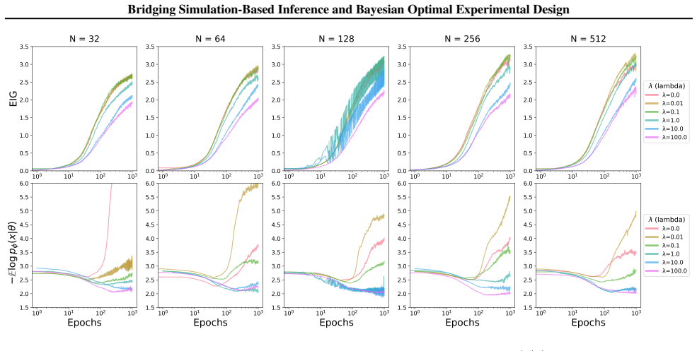
The object that carries the argument is the InfoNCE mutual-information bound re-expressed with a normalizing flow in place of the usual classifier critic: $$L_{NCE}(\xi,\phi;L) = \mathbb{E}\left[\log\frac{p_\$\varphi$(y|\theta_0,\xi)}{\frac{1}{1+L}\sum_{\ell=0}^{L}p_\$\varphi$(y|\theta_\ell,\xi)}\right],$$ where the expectation is over $p(\theta_0)p(y|\theta_0,\xi)p(\theta_{1:L})$ and $p_\phi$ is a conditional normalizing flow (a neural spline flow in the experiments). The flow does two jobs at once: as a normalized density it makes the bracketed ratio a valid lower bound on $I(\theta;y|\xi)$, and as a pathwise generative model $y = f^{-1}(u;\theta,\xi)$ it lets gradients with respect to the design $\xi$ be computed by backpropagation through the flow, so no gradient ever needs to pass through the simulator. Theorem 3.1 identifies the $\phi$ that maximizes this bound with the $\phi$ that minimizes the likelihood KL divergence plus a marginal-likelihood KL term. The refinement $L_{NCE\text{-}\lambda}$ appends $\lambda\log p_\phi(y|\theta_0,\xi)$, and the optimizer acts on the parameters of a truncated-normal design distribution rather than on the designs themselves, with an annealing width schedule and design checkpoints to escape reward-poor regions and local minima.
What would settle it
On a simulator with a closed-form likelihood and marginal — the paper's noisy linear model is one — fit two surrogates: one by maximizing the InfoNCE bound with a small contrastive batch, and one by directly minimizing the likelihood KL divergence of Equation (3). If the two optima do not converge to the same density as the contrastive batch size $L$ grows, Theorem 3.1 is false as stated. A second check on the same model: run SBI-BOED where the optimal design is known in closed form; if the selected design does not approach it as training steps and $L$ grow, the gradient path through the surrogate is not faithfully optimizing information gain.
Extended reading notes
Core claim
On its own terms, the discovery is that the InfoNCE bound, written with a normalized density estimator as the critic, is simultaneously an objective for likelihood-based SBI and for gradient-based BOED. Concretely, the paper defines $$L_{NCE}(\xi,\phi;L) = \mathbb{E}_{p(\theta_0)p(y|\theta_0,\xi)p(\theta_{1:L})}\left[\log \frac{p_\$\varphi$(y|\theta_0,\xi)}{\frac{1}{1+L}\sum_{\ell=0}^{L}p_\$\varphi$(y|\theta_\ell,\xi)}\right],$$ with $\phi$ parameterizing a normalizing flow $p_\phi(y|\theta,\xi)$, and proves in Theorem 3.1 that maximizing this lower bound over $\phi$ is equivalent to minimizing $\mathbb{E}_{p(\theta)}D_{KL}(p(y|\theta,\xi)\|p_\phi(y|\theta,\xi))$ together with the marginal-divergence term $\mathbb{E}_{p(y|\xi)}D_{KL}(p(y|\xi)\|p_\phi(y|\xi))$. Because the flow's sampling path $y = f^{-1}(u;\theta,\xi)$ is differentiable in the design $\xi$, gradients for design updates flow through the surrogate, so the simulator itself never needs to be differentiable. The paper's regularized objective $L_{NCE\text{-}\lambda}$ adds $\lambda\log p_\phi(y|\theta_0,\xi)$, and its design-distribution trick optimizes the parameters of a truncated normal over designs with an annealing width, with checkpoints that keep the best design found. Empirically, SBI-BOED reports lower L-C2ST calibration error and smaller median prediction distance than MINEBED-BO and iDAD on both the SIR and BMP tasks, while its expected information gain is lower on SIR but higher on BMP — evidence, the paper argues, that information gain and trustworthy inference should be evaluated separately.
Load-bearing premise
The bridge between the two fields stands on one substitution: in the proof of Theorem 3.1 the true distribution of simulated data is replaced by an average over a finite batch of surrogate-likelihood samples, and the proof marks that step as approximately equal; if this substitution is not accurate, maximizing the InfoNCE bound is no longer provably the same as fitting the likelihood, and the method's value rests on its empirical results alone.
Editorial extensions
If this is right
- Black-box simulators that cannot be differentiated become optimizable for experimental design: the gradient path runs through the surrogate flow, so the design update requires only simulator samples, not simulator gradients.
- A single trained object serves both purposes at once — the amortized likelihood used for posterior inference is the same surrogate whose gradients selected the design — removing the separate critic/design-policy split in earlier gradient-based BOED methods.
- Designs with the highest expected information gain are not automatically the ones that yield the best-calibrated posteriors; on the SIR and BMP tasks the lower-EIG SBI-BOED surrogates beat the higher-EIG baselines on L-C2ST and median prediction distance.
- The $\lambda$ dial lets a practitioner choose a working point on the trade-off between a tight mutual-information bound and an accurate likelihood surrogate, which matters most in high-dimensional design spaces where the unregularized objective is unstable.
- Any generative model with an evaluable likelihood or likelihood lower bound (diffusion models, flow matching) can substitute for the normalizing flow in the same procedure.
Reading between the lines
- The equivalence in Theorem 3.1, if exact, implies the converse direction the paper does not pursue: ordinary likelihood-based SBI training is implicitly a design-optimization procedure, so calibration-aware objectives could be imported into plain SBI practice even when no experiment is being planned.
- Appendix B.2's bound, $I_{NCE\text{-}\lambda} \le \log(L+1) - \lambda\,\mathbb{E}_{\theta}H(y|\theta,\xi)$, suggests a testable shortcut: the surrogate's conditional entropy could serve as a cheap acquisition function during design search, replacing the separate EIG estimate used for checkpoints.
- The paper's dissociation between EIG and calibration, if it replicates across more tasks and seeds, would push the field toward reporting calibration metrics alongside information gain in every BOED evaluation, since an overconfident posterior can accompany a high-information design.
- Because the surrogate is trained on prior samples, its accuracy should degrade as the posterior concentrates over successive design rounds; reusing posterior samples as a proposal distribution for the next round, which the paper notes but does not implement, is the natural fix for the conservative SBC curves it reports.
Editorial analysis
A structured set of objections, weighed in public.
Referee Report
Summary. The paper proposes SBI-BOED, a method for jointly training an amortized normalizing-flow likelihood surrogate and optimizing experimental designs in simulation-based inference without differentiating through the simulator. The method maximizes an InfoNCE-style lower bound on mutual information (Eq. 6), adds a likelihood regularizer INCE-λ (Eq. 8), and uses a truncated-normal design distribution with checkpoints to stabilize design optimization. Experiments on a noisy linear model, an SIR epidemic model, and a BMP signaling model compare EIG, L-C2ST calibration, and median posterior prediction distance against MINEBED and iDAD. The central theoretical claim is Theorem 3.1, which asserts equivalence between maximizing the InfoNCE bound and minimizing the sum of the likelihood KL and marginal KL.
Significance. The proposed pipeline is practically appealing: it handles non-differentiable simulators, produces a normalized amortized likelihood, and the use of design distributions and checkpoints addresses a real optimization failure mode. The paper also reports external calibration (L-C2ST) and prediction-distance metrics rather than only EIG, and states that code is available. However, the theoretical bridge in Theorem 3.1 is incorrect as stated, the proof in Appendix A.1 relies on an unjustified finite-sample replacement, and the empirical comparisons rest on three seeds and method-specific EIG estimators. The core idea may still be salvageable, but the manuscript in its current form substantially overclaims.
major comments (4)
- [§3.1, Appendix A.1, Eq. (7)] Theorem 3.1 is not correct as stated. For Eq. (6), the L→∞ limit is E_{p(θ,y)} log p_φ(y|θ) − E_{p(y)} log p_φ(y), where p_φ(y)=E_{p(θ)}p_φ(y|θ). Adding and subtracting the true conditional entropy yields I(θ;y) − D_KL(p(y|θ)∥p_φ(y|θ)) + D_KL(p(y)∥p_φ(y)). Since I is independent of φ, maximizing the InfoNCE bound is equivalent to minimizing D_KL(p(y|θ)∥p_φ(y|θ)) − D_KL(p(y)∥p_φ(y)), not the sum in Eq. (7). The error originates in Appendix A.1: after Eq. (21), E_{p(y)} log[ˆp(y)/p(y)] = −D_KL(p(y)∥ˆp(y)), but Eq. (22) replaces it with −E_{ˆp(y)}D_KL(ˆp(y)∥p(y)), reversing the direction and the expectation; Eq. (23) then treats E_{ˆp(y)}log p(y) as constant even though ˆp depends on φ. This is not a finite-L artifact; it survives at L=∞. The theorem and the remark about reverse-KL bias in Appendix A.1 need to be corrected or the theoretical claims substantially restricted.
- [Appendix B.1, Eq. (30)] The λ analysis in Appendix B.1 is not a valid KL-divergence calculation: Eq. (30) defines D_KL(p(y|θ)∥p_φ(y|θ)^{1−λ}), where p_φ^{1−λ} is generally unnormalized, so it is not a divergence and cannot be used to conclude that λ>0 yields 'broad coverage' and λ<0 yields 'mode-seeking'. The empirical λ sweeps in Sections 5.1 and 5.3 may still be valid evidence, but the paper should either provide a corrected analysis of the regularized objective or present λ as a purely heuristic regularizer.
- [Table 1, Sections 5.3–5.4] The EIG column in Table 1 is not comparable across methods because each method estimates EIG with its own estimator: MINEBED uses the MINE bound, iDAD uses InfoNCE with a critic, and SBI-BOED uses the INCE-λ surrogate. Differences as small as 0.02–0.2 can easily be estimator bias. Therefore the statement that iDAD and differentiable MINEBED 'achieve the best information gain' is not supported; a common EIG estimator (e.g., a high-L InfoNCE or nested Monte Carlo estimate evaluated on the same samples) should be applied to all final designs.
- [Sections 5.3–5.4, Table 1] The empirical claims of 'notable improvements in inference' rest on 3 seeds and T=2 (SIR) or T=3 (BMP) design rounds. For SIR, SBI-BOED's EIG is 1.01–1.63 versus 2.67–2.69 for the benchmarks, and the calibration differences are within one standard error for several rows (e.g., 0.03±0.01 vs 0.07±0.05). More seeds, more design rounds, and ideally a shared evaluation protocol are needed before claiming state-of-the-art calibration and accuracy.
minor comments (4)
- [Section 5.3] There is a typo, 'rouglhy' should be 'roughly'.
- [Section 3.1, Eq. (5)] The displayed inequality in Eq. (5) is not valid in general: log[exp(g0)/(L^{-1}\sum_{\ell=1}^L exp g_\ell)] ≤ log[exp(g0)/((L+1)^{-1}\sum_{\ell=0}^L exp g_\ell)] holds only when exp(g0) ≤ L^{-1}\sum_{\ell=1}^L exp(g_\ell); otherwise the direction is reversed. Since this inequality is not needed once p_φ is a normalized density, either remove it or state the condition.
- [Algorithm 1, line 9] The checkpoint condition 'if EIG ξ > EIGξ∗' uses the surrogate's own EIG estimate; this should be clearly described as an online model-selection heuristic, and the sensitivity of the final design to this choice should be discussed.
- [Figure 2] The caption says 'moving average over 10 different random seed initializations,' while Table 1 reports 3 seeds; please clarify the number of seeds used for each figure and table.
Circularity Check
No substantive circularity in the derivation; the only self-referential element is that the EIG metric for SBI-BOED is the training objective itself, while the independent calibration and accuracy claims stand.
-
fitted input called prediction
[Section 3.2, Eqs. (9)-(10); Section 5.3, Table 1]
"EIGi refers to the theoretical information gain expected from a single sample realization under design ξi, based on the current parameterization of the likelihood. It quantifies the information gain computed from a possible outcome as EIGi(ψ, ϕ, L, λ) = E[ log pϕ(yi|θ0, ξi)1+λ / (1/(1+L) Σℓ=0^L pϕ(yi|θℓ, ξi)) ], (10)"
Equation (10) is the same functional as the INCE-λ objective in Eq. (9), with the same learned density pϕ and the same contrastive denominator. Because pϕ is trained by maximizing Eq. (9), the quantity reported as EIG for SBI-BOED is the training objective itself, so the EIG comparison in Table 1 is in-sample and the BMP EIG advantage is partly by construction. This does not affect the independent L-C2ST and median-distance evaluations, which are computed against simulator ground truth, and the paper's own SIR results show SBI-BOED with lower EIG than the benchmarks, limiting the scope of the self-referentiality.
full rationale
The paper's central derivation is not circular: SBI-BOED trains a normalizing-flow likelihood surrogate by maximizing the InfoNCE lower bound on mutual information and uses pathwise gradients to optimize designs, a standard variational procedure. The calibration and predictive-accuracy evaluations (L-C2ST and median distance) are external to the training objective and provide independent evidence for the paper's main empirical claims. There are no self-citations, imported uniqueness theorems, or ansatz-smuggling citations that are load-bearing. The Appendix A.1 proof of Theorem 3.1 contains an apparent sign error in the marginal-KL term and an explicit '≈' replacement of the true marginal by the model marginal; however, those are correctness or rigor concerns, not circularity, because the claimed equivalence is not obtained by defining one side in terms of the other. The only identifiable circular element is the EIG metric: Eq. (10) relabels the INCE-λ objective as EIG, so Table 1's EIG column for SBI-BOED is an in-sample measure rather than an independent estimate. This is a moderate self-referentiality in one benchmark metric, but the paper de-emphasizes EIG by explicitly noting that better EIG does not imply better downstream prediction, and the external metrics carry the central claims. Overall circularity score: 2.
Assumptions & free parameters
free parameters (3)
- λ (INCE-λ regularization weight) =
evaluated at 0, 0.01, 0.1, 1.0; no automatic selection
- Design distribution std-dev schedule (σ_start, σ_end, ρ) and truncation bounds [α, β] =
σ_start/σ_end/ρ set per experiment (Table 2 in Appendix D); bounds [α,β] per task
- Number of contrastive samples L =
50 (linear), 255 (SIR), 127 (BMP)
assumptions (5)
- standard math InfoNCE objective is a valid lower bound on MI when the critic is a normalized density p_φ(y|θ,ξ)
- ad hoc to paper The marginal approximation ˆp(y) from L contrastive samples is close enough to the true marginal p(y) to justify the KL equivalence
- domain assumption The normalizing flow p_φ has enough capacity and is trained with enough data to faithfully represent the true likelihood over the design space
- standard math Conditioning on a random design ξ drawn from p(ξ) preserves a valid MI objective
- domain assumption Observations are i.i.d. so the likelihood factorizes into a product over design rounds
Cite this review
Pith. "Pith review of Optimizing Likelihoods via Mutual Information: Bridging Simulation-Based Inference and Bayesian Optimal Experimental Design." pith.science (2026). https://pith.science/paper/7HCLSZAK
@misc{pith2026250208004,
  author       = {Pith},
  title        = {Pith review of: Optimizing Likelihoods via Mutual Information: Bridging Simulation-Based Inference and Bayesian Optimal Experimental Design},
  year         = {2026},
  howpublished = {\url{https://pith.science/paper/7HCLSZAK}},
  note         = {Machine review of arXiv:2502.08004}
}
read the original abstract
Simulation-based inference (SBI) is a method to perform inference on a variety of complex scientific models with challenging inference (inverse) problems. Bayesian Optimal Experimental Design (BOED) aims to efficiently use experimental resources to make better inferences. Various stochastic gradient-based BOED methods have been proposed as an alternative to Bayesian optimization and other experimental design heuristics to maximize information gain from an experiment. We demonstrate a link via mutual information bounds between SBI and stochastic gradient-based variational inference methods that permits BOED to be used in SBI applications as SBI-BOED. This link allows simultaneous optimization of experimental designs and optimization of amortized inference functions. We evaluate the pitfalls of naive design optimization using this method in a standard SBI task and demonstrate the utility of a well-chosen design distribution in BOED. We compare this approach on SBI-based models in real-world simulators in epidemiology and biology, showing notable improvements in inference.
Figures


Figures from the paper (5 more)


Forward citations
Cited by 1 Pith paper
-
Identifying Informative Environments for Cognition Parameter Inference via Bayesian Experimental Design
On Mouselab-MDP, amortized Bayesian experimental design ranks planning environments by expected information gain almost as well as exact Monte Carlo BED, and no single environment wins on all objectives.
Reference graph
Works this paper leans on
-
[3]
9 Bridging Simulation-Based Inference and Bayesian Optimal Experimental Design S
arXiv: 2002.08129 Publication Title: arXiv. 9 Bridging Simulation-Based Inference and Bayesian Optimal Experimental Design S. Kleinegesse and M. U. Gutmann. Gradient-based Bayesian Experimental Design for Implicit Models using Mutual Information Lower Bounds. May
arXiv 2002
-
[7]
We also found issues with MCMC sampling from the product likelihood in this case but our technique does show how to simultaneously optimize designs and a likelihood in a non-differentiable scientific simulator. However, we would 18 Bridging Simulation-Based Inference and Bayesian Optimal Experimental Design 0 20 40 60 80 100 Measurement Time 0 50 100 150 ...
work page 2019
-
[10]
bound has been used in BOED in Kleinegesse and Gutmann (2021); Ivanova et al. (2021). Adjusting the bound from Ivanova et al. (2021), LNWJ(ξ, ϕ) := Ep(θ)p(y|θ,ξ) [gϕ(y, θ)] − e−1 Ep(θ)p(y|ξ) [exp(gϕ(y, θ))] , (47) where gϕ is a classifier that returns the probability that y belongs to θ. This function has lower bias than the InfoNCE bound but higher varia...
work page 2021
-
[500]
For the model parameters β and γ, we use log-normal priors such that p(β) = Lognorm(0.50, 0.502) and p(γ) = Lognorm(0.10, 0.502). Since solving the SDE is time-consuming, we pre-simulate data on a time grid in each round and access the relevant data regions during training. BMP Experiment Details The BMP signaling pathway can be described by mass action k...
work page 2022
-
[1994]
the normalizing constant is difficult to approximate. Greenberg et al. (2019) alternatively proposed to approximate the intractable normalizing constant by replacing the integral with a summation term that takes draws of the parameters from a proposal setΘ such that the posterior is approximately: p(θ|y) ≈ pϕ(θ|y)/p(θ)P θ′∈Θ pϕ(θ′|y)/p(θ′) . (44) Applying...
work page 2019
-
[2007]
as a closed-box solver. E. Expanded Two Moons Results We analyze the mode collapse of the likelihood-based two moons posterior prediction related to the MI optimization. We also show a Simulation-Based Calibration (SBC) (Talts et al., 2020; Hermans et al.,
work page 2020
-
[2010]
ISSN 1557-9654. doi: 10.1109/tit.2010.2068870. G. Papamakarios and I. Murray. Fast ϵ-free inference of simulation models with bayesian conditional density esti- mation. In Advances in Neural Information Processing Systems, volume 29, pages 1028–1036,
- [2015]
Show all 15 references
-
[2016]
An alternative method was 15 Bridging Simulation-Based Inference and Bayesian Optimal Experimental Design developed by Greenberg et al
or variance (Lueckmann et al., 2017). An alternative method was 15 Bridging Simulation-Based Inference and Bayesian Optimal Experimental Design developed by Greenberg et al. (2019) to recover the unbiased posterior, p(θ|y) ≈ pϕ(θ|y)/p(θ) Zϕ(y) (43) by calculating the normalizi...
2019
-
[2017]
11 Bridging Simulation-Based Inference and Bayesian Optimal Experimental Design A. Mutual Information-Based Likelihood Optimization Derivation & Proofs We provide a derivation and proof of how optimizing a lower bound of the mutual information is the same as minimizing the KL ...
2024
-
[2019]
This approximates the marginal likelihood with a root sample from the prior p(θ0), and samples from an approximate posterior θi ∼ q(θ|y)
suggest simultaneously optimizing a posterior distribution at the same time as a likelihood via Likelihood-Free Adaptive Contrastive Estimation (LF-ACE). This approximates the marginal likelihood with a root sample from the prior p(θ0), and samples from an approximate posterio...
2023
-
[2020]
Devlin, M.-W
J. Devlin, M.-W. Chang, K. Lee, and K. Toutanova. BERT: Pre-training of deep bidirectional transformers for lan- guage understanding. In Proceedings of the 2019 Con- ference of the North American Chapter of the Associa- tion for Computational Linguistics: Human Language Techno...
2019
-
[2021]
arXiv: 2105.04379. I. Kobyzev, S. Prince, and M. Brubaker. Normalizing Flows: An Introduction and Review of Current Methods. IEEE Transactions on Pattern Analysis and Machine Intelli- gence, Aug
-
[2023]
Glaser, M
P. Glaser, M. Arbel, S. Hromadka, A. Doucet, and A. Gret- ton. Maximum likelihood learning of unnormalized models for simulation-based inference. arXiv preprint arXiv:2210.14756,
-
[2024]
Their results hint at using a bound on the MI to optimize a likleihood-to-evidence ratio, and saw increasing EIG (lower bound of MI) with increasing number of contrastive samples
noted the connection between Equation (46) and the NWJ bound, and gave a tighter bound on the NWJ-based bound using their SBI-based CRE method. Their results hint at using a bound on the MI to optimize a likleihood-to-evidence ratio, and saw increasing EIG (lower bound of MI) ...
2020
Reviewed August 8, 2026 · model on record in the stance chip above.
Discussion (0). Continue with ORCID to comment.