REVIEW 4 major objections 6 minor 17 references
View management for lifelong visual maps
T0 review · 4 major / 6 minor · reviewed 2026-08-14 · deepseek-v4-flash
Pith's one-line read A scoring rule based on view observation history can prune a lifelong visual SLAM map down to roughly 300 views in home-sized environments, preserving relocalization across changing lighting and layout rather than letting the map grow…
desk verdict A useful online view-pruning idea for lifelong SLAM, but Algorithm 1 as printed cannot prune any views, so the paper needs a major fix before its results can be trusted. read the letter →
The pith
A machine-rendered reading of the paper's core claim, the machinery that carries it, and where it could break.
The reading
What carries the argument
The load-bearing mechanism is a two-stage pruning rule driven by observation statistics. First, each pre-existing view receives a score from a weighted combination of a relocalization flag, current-run observation count normalized by the maximum observation count, and run-observation count normalized by the total number of runs; views above the score threshold are kept. Second, the remaining deletion candidates are sorted by score and removed only if the number of neighboring views in a voxel of size (x, y, θ) is at least a nearest-neighbor threshold, which keeps the surviving views spatially and angularly uniform. The algorithm runs in about 300 ms for systems with up to 500 views on a 1.2 GHz quad-core processor, which is what makes on-agent lifelong view management feasible.
What would settle it
Rerun the same sequential log experiments with pruned and unpruned maps while recording absolute pose error against ground truth and per-frame CPU time for view observation; if the capped map shows larger trajectory error or no CPU savings, the claim that pruning preserves speed and accuracy is false. A targeted version would build a map component whose relocalization depends on one rarely observed view and test whether the score deletes it, blocking relocalization entirely.
Extended reading notes
Core claim
The central discovery is that a view's future relocalization value can be summarized by three observation statistics accumulated over runs: whether the view was ever used to relocalize, its observation frequency in the current run relative to the most-observed view, and the fraction of runs in which it was observed at least once. A weighted sum of these statistics forms a view score; views below a score threshold become deletion candidates, and a nearest-neighbor constraint then prevents pruning views whose spatial and angular neighborhood would become too sparse. The authors demonstrate over 100 sequential runs in four environments that this procedure keeps the map usable while capping view count, and they identify parameter settings that balance growth suppression against relocalization performance. The result, as stated in the paper, is an algorithm capable of limiting the growth of the number of views in the SLAM system without compromising its ability to relocalize despite appearance changes.
Load-bearing premise
The load-bearing premise is that the three relocalization statistics—distance between cross-observations, fraction of cross-observed frames, and relocalization distance—are faithful proxies for true localization quality; the paper states that it does not show data on speed or pose accuracy after pruning, so if those proxies miss real degradation, the claim of uncompromised performance is unsupported.
Editorial extensions
If this is right
- In environments under 1000 square feet, the view count can be kept near 300 instead of growing to about 1500, with the stabilized count reached after roughly 5 to 10 runs.
- Relocalization into a previously saved map remains possible across lighting changes and moved furniture, as measured by relocalization distance and fraction of cross-observed frames over 100 runs.
- The pruning rule can run online on the robot's own processor, so lifelong map maintenance does not require an offline, server-side summarization step.
- The algorithm's parameters can be tuned sequentially: first score weights, then nearest-neighbor voxel size and threshold, using the paper's reported growth and relocalization criteria.
- Because views that are never observed again are removed, the map naturally forgets scenes that are no longer observable and keeps the view distribution uniform.
Reading between the lines
- A natural transfer would be to other keyframe- or view-based SLAM systems: the score and neighbor definitions are generic, but the weights and voxel size would need recalibration to each system's observation behavior.
- The pruning rule implicitly acts as an appearance-based forgetting mechanism; in a sufficiently long deployment it should keep only the views compatible with the environment's current lighting and layout, which could be tested by comparing the surviving views with the current scene appearance.
- A missing piece the paper acknowledges is direct evidence on speed and pose accuracy; an experiment that measures absolute trajectory error and per-frame CPU time before and after pruning would either confirm or undercut the claim that bounded views mean acceptable performance.
- The uniform-distribution constraint could also be repurposed as a map-quality metric, for example to detect regions of the environment that are under-observed and may need deliberate exploration.
Signed reviews
Editorial analysis
A structured set of objections, weighed in public.
Referee Report
Summary. The paper proposes an online view-management (pruning) algorithm for lifelong visual SLAM on resource-constrained robots. Each view is scored as a weighted combination of whether it was used for relocalization, how often it was observed in the current run, and how many previous runs observed it; views with low scores are candidates for deletion, subject to a nearest-neighbor constraint intended to preserve a uniform spatial distribution of views. Experiments on logs from four environments over 100 sequential runs report that the number of views stabilizes near 300, while relocalization distance, fraction of cross-observed frames, and distance between cross-observations remain at levels similar to those used during parameter tuning. The paper concludes that the algorithm limits view growth without compromising relocalization ability despite appearance changes.
Significance. If the claims hold, the paper addresses a real practical problem: view growth in lifelong visual SLAM on memory- and compute-constrained platforms. The algorithm is simple, online, and does not require offline computation or a server connection, which differentiates it from summary-map and experience-based approaches. The paper also defines concrete relocalization metrics and reports results over many runs in multiple environments, which is a strength. The authors are honest about omitted CPU and accuracy data. However, the central experimental claim is not fully supported as written because of an internal inconsistency in the pseudocode and the absence of a no-pruning control on the same metrics; the parameter-selection procedure also overlaps with the reported success metrics. For these reasons the manuscript needs substantive revision before it can be accepted.
major comments (4)
- [§IV-B, Algorithm 1] Algorithm 1 as printed cannot delete any view when NN_THRESHOLD is at least 1. Line 10 initializes D to the empty set; line 12 keeps any v in Vdelete for which numNearestNeighbors(v,D) < NN_THRESHOLD. The first candidate therefore has zero neighbors in D and is moved to Vkeep, D remains empty, and by induction every candidate is kept, so Vdelete is returned empty. The prose accompanying the algorithm says the check should use 'the number of nearby views,' not the number of nearby views already marked for deletion. This is an internal inconsistency: §V-D reports stabilized view counts with NN_THRESHOLD=5 and Table II tunes NN_THRESHOLD over 1–5, outcomes that are impossible under the printed algorithm. The pseudocode needs to be corrected (for example, by counting neighbors in Vkeep or in all of V) so that the reported experiments are reproducible.
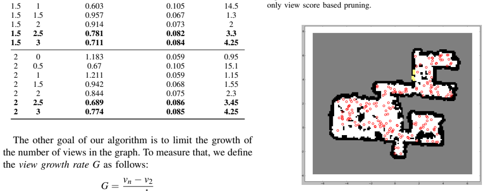
- [§V-D, Fig. 8] The central claim that pruning does not compromise relocalization is not supported by a no-pruning control on the same metrics. The 100-run experiments report view counts, relocalization distance, fraction of cross-observed frames, and distance between cross-observations only for the full algorithm. The baseline values cited in §V-C (average relocalization distance 11.78 m, growth rate 4.25) are for score-based pruning without the nearest-neighbor constraint, not for the unpruned system. Without a same-protocol, no-pruning comparison on the relocalization metrics, the conclusion in §VI that the algorithm limits growth 'without compromising its ability to relocalize' is not established.
- [§V-B and §V-D, Tables I-II] The parameters W1, W2, W3, SCORE_THRESHOLD, NN_THRESHOLD, and NN_VOXEL_SIZE are selected on environment A using thresholds on the distance between cross-observations, fraction of cross-observed frames, and growth rate (Table I), and on relocalization distance and growth rate (Table II). The same metrics are then reported as the success criteria of the 100-run evaluation, including for environment A itself. This overlap between tuning and evaluation leaves the reported numbers open to overfitting; the paper should either show that the chosen parameters work across a range of nearby settings, or evaluate on environments excluded from parameter selection.
- [§V, first paragraph] The manuscript explicitly states that no CPU-utilization or localization-accuracy data are shown ('we do not show any data related to this'). Since the motivation in §I and §III is to prevent unacceptable speed and accuracy degradation on a resource-constrained platform, the reported relocalization metrics are only indirect evidence. If those metrics are not a faithful proxy for end-to-end pose accuracy or for the time cost of view observation, the claim that performance is 'not compromised' remains unverified. Please either provide direct measurements on the target platform or temper the conclusion accordingly.
minor comments (6)
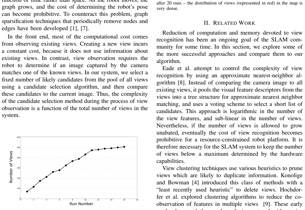
- [§I, Fig. 3] The axes in Fig. 3 are unlabeled and the caption does not state the units or the number of runs; please add axis labels and a caption describing what is plotted.
- [§IV-B, text after Algorithm 1] The sentence 'the view from Vdelete and added to Vkeep' is missing a verb; it should read 'the view is moved from Vdelete and added to Vkeep.'
- [Abstract] There is an extra space before the period in 'sub-linear .'; please remove it.
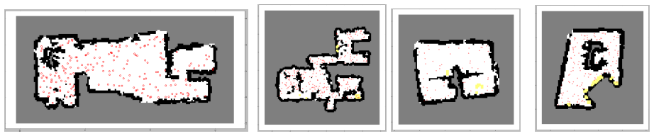
- [§V-D] The statements that view counts 'usually stabilize within 300' and that this holds for 'environments below 1000 ft²' are informal; please report the mean and range across the four environments and define what 'usually' means quantitatively.
- [§V-C, Table II] The sentence listing suitable parameter sets ends with '(5, 1m, 1m, 2 rad)' while the final experiments use NN_THRESHOLD=5 with voxel (1m, 1m, 2 rad); the ordering of the list makes this easy to misread, so please present the chosen parameter set explicitly in the text.
- [§V-D] The reported runtime of around 300 ms for up to 500 views is not attributed to a specific component; please clarify whether this is the full pruning pass or only the nearest-neighbor check.
Circularity Check
No significant circularity: parameter tuning on one environment is in-sample, but validation on three held-out environments gives independent support; the Algorithm 1 pseudocode bug is a reproducibility flaw, not circularity.
full rationale
I found no circularity as defined by the review criteria. The algorithm's score function and nearest-neighbor constraint are specified independently of the evaluation metrics: the view score combines relocalization use, current-run observation ratio, and historical observation ratio, while the NN constraint enforces spatial uniformity. The parameters are tuned on Environment A logs using the same relocalization metrics that later appear in the 100-run evaluation (Tables I-II and Figs. 8-11), which is an in-sample tuning weakness for Environment A; however, the paper also validates on Environments B, C, and D, which were not used for tuning, so the central claim that view growth is limited without compromising relocalization has independent empirical content and is not forced by construction. The self-citations ([1], [7]) are background references and are not load-bearing for the pruning claim. The statement in Section V that speed and pose-accuracy data are not shown ('we do not show any data related to this') is an acknowledged limitation, not circularity. Separately, Algorithm 1 as printed is internally inconsistent: D is initialized empty, and the condition numNearestNeighbors(v, D) < NN_THRESHOLD keeps every view, so the printed pseudocode cannot prune any views. This is a serious correctness and reproducibility flaw, but it is not circularity: the reported conclusion is unsupported by the printed algorithm rather than equivalent to its inputs.
Assumptions & free parameters
free parameters (5)
- W1, W2, W3 (view score weights) =
1.5, 1, 3
- SCORE_THRESHOLD =
1.375 (Section V-D); Table I uses 0.25 times max score
- NN_THRESHOLD =
5
- NN_VOXEL_SIZE =
(1 m, 1 m, 2 rad)
- MIN_VIEWS =
25
assumptions (4)
- domain assumption Relocalization distance, fraction of cross-observed frames, and distance between cross-observations are sufficient proxies for localization performance.
- domain assumption The graph-based SLAM system with views, components, and pose-to-view edges behaves as described by Eade et al.
- domain assumption A view that is rarely observed and that has many similar-orientation neighbors can be removed without hurting future relocalization.
- domain assumption Parameters tuned on environment A generalize to other environments.
Cite this review
Pith. "Pith review of View management for lifelong visual maps." pith.science (2026). https://pith.science/paper/7JTHYPEH
@misc{pith2026190803605,
  author       = {Pith},
  title        = {Pith review of: View management for lifelong visual maps},
  year         = {2026},
  howpublished = {\url{https://pith.science/paper/7JTHYPEH}},
  note         = {Machine review of arXiv:1908.03605}
}
read the original abstract
The time complexity of making observations and loop closures in a graph-based visual SLAM system is a function of the number of views stored. Clever algorithms, such as approximate nearest neighbor search, can make this function sub-linear. Despite this, over time the number of views can still grow to a point at which the speed and/or accuracy of the system becomes unacceptable, especially in computation- and memory-constrained SLAM systems. However, not all views are created equal. Some views are rarely observed, because they have been created in an unusual lighting condition, or from low quality images, or in a location whose appearance has changed. These views can be removed to improve the overall performance of a SLAM system. In this paper, we propose a method for pruning views in a visual SLAM system to maintain its speed and accuracy for long term use.
Figures


Figures from the paper (8 more)



Reference graph
Works this paper leans on
-
[1]
Monocular graph SLAM with complexity reduction,
E. Eade, P. Fong, and M. E. Munich, “Monocular graph SLAM with complexity reduction,” IEEE IROS, pp. 3017–3024, 2010
work page 2010
-
[2]
K. Konolige, J. Bowman, J. Chen, P. Mihelich, M. Calonder, V . Lepetit, and P. Fua, “View-based maps,”The International Journal of Robotics Research, vol. 29, no. 8, pp. 941–957, 2010
work page 2010
-
[3]
iRobot’s new Ava 500 puts robotics in heart of the enterprise,
“iRobot’s new Ava 500 puts robotics in heart of the enterprise,” https://www.forbes.com/sites/jenniferhicks/2013/06/ 10/irobots-new-ava-500-puts-robotics-in-heart-of-the-enterprise/ #3506cd972e1b, accessed: 2018-09-14
work page 2013
-
[4]
K. Konolige and J. Bowman, “Towards lifelong visual maps,” in IEEE IROS, 2009, pp. 1156–1163
work page 2009
-
[5]
Towards a robust back-end for pose graph slam,
N. S ¨underhauf and P. Protzel, “Towards a robust back-end for pose graph slam,” in IEEE ICRA , May 2012, pp. 1254–1261
work page 2012
-
[6]
Factor graphs for robot perception,
F. Dellaert and M. Kaess, “Factor graphs for robot perception,” F oundations and Trends in Robotics, vol. 6, no. 1-2, pp. 1–139, 2017. [Online]. Available: http://dx.doi.org/10.1561/2300000043
-
[7]
Fast nonlinear approximation of pose graph node marginalization,
D.-N. Ta, N. Banerjee, S. Eick, S. Lenser, and M. Munich, “Fast nonlinear approximation of pose graph node marginalization,” in IEEE ICRA, May 2018
work page 2018
-
[8]
Fast approximate nearest neighbors with automatic algorithm configuration,
M. Muja and D. G. Lowe, “Fast approximate nearest neighbors with automatic algorithm configuration,” in In VISAPP International Conference on Computer Vision Theory and Applications , 2009, pp. 331–340
work page 2009
Show all 17 references
-
[9]
Lifelong localization of a mobile service-robot in everyday indoor environments using omnidi- rectional vision,
S. Hochdorfer, M. Lutz, and C. Schlegel, “Lifelong localization of a mobile service-robot in everyday indoor environments using omnidi- rectional vision,” in IEEE International Conference on Technologies for Practical Robot Applications (TEPRA) , November 2009
2009
-
[10]
Predicting matchabil- ity,
W. Hartmann, M. Havlena, and K. Schindler, “Predicting matchabil- ity,” in IEEE CVPR , June 2014, pp. 9–16
2014
-
[11]
Saliency-based keypoint selection for fast object detection and matching,
S. Buoncompagni, D. Maio, D. Maltoni, and S. Papi, “Saliency-based keypoint selection for fast object detection and matching,” Pattern Recognition Letters , vol. 62, pp. 32–40, 2015
2015
-
[12]
Erasing bad memories: agent-side summarization for long- term mapping,
M. Dymczyk, T. Schneider, I. Gilitschenski, R. Siegwart, and E. Stumm, “Erasing bad memories: agent-side summarization for long- term mapping,” in IEEE IROS, October 2016
2016
-
[13]
Summary maps for lifelong visual localization,
P. M ¨uhlfellner, M. B ¨urki, M. Bosse, W. Derendarz, R. Philippsen, and P. Furgale, “Summary maps for lifelong visual localization,” Journal of Field Robotics , vol. 33, no. 5, pp. 561–590, 2015. [Online]. Available: https://onlinelibrary.wiley.com/doi/abs/10.1002/rob.21595
2015 doi
-
[14]
Appearance-based landmark selection for efficient long-term visual localization,
M. B ¨urki, I. Gilitschenski, E. Stumm, R. Siegwart, and J. Nieto, “Appearance-based landmark selection for efficient long-term visual localization,” in IEEE IROS, Oct 2016, pp. 4137–4143
2016
-
[15]
Keep it brief: Scalable creation of compressed localization maps,
M. Dymczyk, S. Lynen, M. Bosse, and R. Siegwart, “Keep it brief: Scalable creation of compressed localization maps,” in IEEE IROS , Sep. 2015, pp. 2536–2542
2015
-
[16]
Practice makes perfect? managing and leveraging visual experiences for lifelong navigation,
W. Churchill and P. Newman, “Practice makes perfect? managing and leveraging visual experiences for lifelong navigation,” in IEEE ICRA , May 2012, pp. 4525–4532
2012
-
[17]
Experience-based navigation for long-term localisation,
——, “Experience-based navigation for long-term localisation,” The International Journal of Robotics Research , vol. 32, no. 14, pp. 1645–1661, 2013. [Online]. Available: https://doi.org/10.1177/ 0278364913499193
2013
Reviewed August 14, 2026 · model on record in the stance chip above.
Discussion (0). Continue with ORCID to comment.