REVIEW 4 major objections 4 minor 41 references
Machine learning and Kolmogorov analysis to reveal gravitational lenses
T0 review · 4 major / 4 minor · reviewed 2026-08-14 · deepseek-v4-flash
Pith's one-line read The paper claims that the Kolmogorov stochasticity parameter can flag sub-regions containing gravitational-lens arcs, and that PCA classification then labels the retrieved objects as lens candidates.
desk verdict A transparent but under-validated feasibility study: the KSP prefilter is sensible, but the lens-detection claim rests on one tuned field. read the letter →
The pith
A machine-rendered reading of the paper's core claim, the machinery that carries it, and where it could break.
The reading
What carries the argument
The load-bearing object is the Kolmogorov stochasticity parameter, $\lambda_n = \sqrt{n}\,\sup_x |F_n(x)-F(x)|$, where $F_n$ is the empirical distribution of pixel intensities in a sub-region and $F$ is the theoretical cumulative distribution. Because the paper first establishes Gaussianity of the SDP.81 data, $F$ is taken to be Gaussian, and each sub-region's $\lambda$ is compared with a map-wide cutoff $\lambda_0 + n\sigma$ with $n=1$ chosen empirically. Two further components carry the rest of the pipeline: a Moore-neighborhood connectivity search that assembles surviving pixels into isolated objects after an intensity cutoff, and principal component analysis of the intensity covariance matrix, whose eigenvalues give an eccentricity $e = (\lambda_1-\lambda_2)/\lambda_1$ and a thickness $\lambda_2$; objects with $e \geq e_{\mathrm{thresh}}$ and $\lambda_2 \leq d_{\mathrm{thick}}$ are kept in the final catalog. The KSP step is what makes the search tractable, restricting detailed shape analysis to a few sub-regions instead of the whole field.
What would settle it
Apply the identical pipeline to a simulated or real lens field whose background is deliberately non-Gaussian, for example Poisson sky noise or a heavy-tailed detector background, and check whether the arc-containing sub-regions still pass the $\lambda_0 + 1\sigma$ filter while noise-only sub-regions do not. A cleaner test of the same assumption is to vary only the multiplier $n$ across a set of fields with known arcs: if no single $n$ keeps the arcs without flooding the candidate list, the empirical threshold rule is the failure point.
Extended reading notes
Core claim
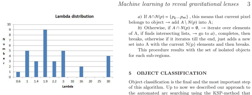
On the paper's own terms, the central discovery is that the Kolmogorov stochasticity parameter (KSP) separates the signal of a lensed object from its surrounding field, and that the separation is enough to drive a fully automated lens-candidate search. In the SDP.81 field, sub-regions containing parts of the lensing arc have anomalously high KSP values against a Gaussian cumulative distribution, with the field's mean KSP around 1.9 and most sub-regions between 0.5 and 2.2. Applying the threshold $\lambda_{\mathrm{thresh}} = \lambda_0 + 1\sigma$ keeps six of thirty-two sub-regions, and every object in the output catalog--with centers, eccentricities, and field numbers--lies inside them. A simulated lens whose arc pixels are only 0.5$\sigma$ above background, invisible to the eye, is still recovered as connected elongated objects. The paper therefore concludes that the method is an automated tool for finding isolated objects and revealing low-significance structures, producing a catalog of possible lensing objects for later inspection.
Load-bearing premise
The whole prefilter rests on the assumption that the SDP.81 intensity field is Gaussian enough for the KSP to be measured against a Gaussian cumulative distribution, and that the empirically chosen one-sigma cutoff will still flag arc-containing sub-regions on other fields; if either fails, real arcs can be discarded before any shape analysis begins.
Editorial extensions
If this is right
- The KSP prefilter can reduce a full survey field to a handful of sub-regions worth detailed lens-shape analysis, saving computation before any pixel-connectivity or PCA work begins.
- Arcs with surface brightness only 0.5 sigma above the background, effectively invisible to the eye, can still be recovered as connected elongated objects, extending the detectable population of lens candidates.
- The pipeline outputs a candidate catalog with object centers, eccentricities, and field numbers, so the surviving candidates can be handed directly to spectroscopic or higher-resolution follow-up.
- Because the eccentricity and thickness thresholds classify by shape alone, the same software can separate elongated arc candidates from more regular galaxies and star clusters in the same field.
- The conclusion suggests the Kolmogorov approach could be applied to other large-survey problems, such as testing the isotropy of gamma-ray burst sky distributions.
Reading between the lines
- A testable extension is to compute the KSP against a locally estimated background distribution on each sub-region instead of a global Gaussian; the threshold would then follow from goodness-of-fit quantiles rather than an empirically chosen $n$, and the prefilter would gain a built-in false-alarm rate.
- The paper notes that spiral arms can be mistaken for arcs; a natural cheap follow-up is to feed the eccentricity candidates into a color or photometric-redshift classifier, since lensed background sources typically have different colors from foreground disk galaxies.
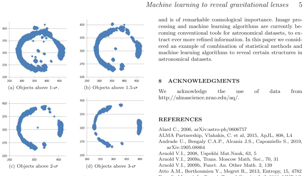
- The visible arc in SDP.81 splits into several fragments at higher intensity cutoffs, which the paper attributes to intensity variation along the arc; the method's own output suggests a merging step over neighboring sub-regions could reconstruct full arcs automatically, something the paper leaves for later grouping.
- Because the KSP responds to any deviation from the assumed background, the pipeline should also flag dust filaments, image artifacts, and other elongated non-lenses; measuring how often such false candidates survive on blank fields would convert the demonstration into a usable survey search.
Signed reviews
Editorial analysis
A structured set of objections, weighed in public.
Referee Report
Summary. The manuscript presents an automated three-stage pipeline for detecting elongated objects, in particular gravitational arcs/lenses, in astronomical images. In the first stage, the image is divided into sub-regions and the Kolmogorov stochasticity parameter (KSP) is computed against a Gaussian theoretical cumulative distribution; sub-regions with lambda above lambda_thresh = lambda_0 + n*sigma are kept, with n chosen empirically. In the second stage, an intensity cut-off and a Moore-neighborhood connected-component labeling algorithm isolate objects. In the third stage, PCA eigenvalues are used to compute eccentricity, and objects satisfying e >= e_thresh and lambda_2 <= d_thick are retained. The pipeline is demonstrated on the SDP.81 strong-lens field (Table 1, Figs. 3-4) and on a simulated low-significance image (Fig. 5), and the authors conclude that the method is an automated search tool for isolated objects that can reveal low-significance lensing structures.
Significance. The paper has some strengths: the pipeline is simple, transparent, and built from standard tools (KSP, connected-component labeling, PCA); the arithmetic appears correctly applied; and the idea of a statistical prefilter to reduce the search space is attractive. The authors also explicitly concede several limitations, such as the empirical choice of thresholds and the possibility of retrieving non-lensing structures. However, the significance of the central claim as presented is limited. The only real-data demonstration is one known lens field, the thresholds are chosen on that same field, and there are no detection metrics such as completeness, false-positive rate, or comparison with existing arc finders (Alard 2006; Seidel & Bartelmann 2007). The simulated test in Fig. 5 shows qualitative retrieval but provides no quantitative recovery statistics. The paper is therefore better characterized as a proof-of-concept than as a validated lens-search method; the general claim that the method 'reveals gravitational lenses' is not yet supported by the evidence.
major comments (4)
- [Section 3, Eq. (2)] The prefilter threshold is lambda_thresh = lambda_0 + n*sigma with n=1, and the text states that this multiplier 'should rather be decided empirically' and that n=1 is chosen because of the data spread. Since the same SDP.81 field is used both to set n and to demonstrate detection, the demonstration does not establish that the prefilter generalizes; a cross-validation test, or a test on an independent field with thresholds fixed in advance, is needed before the method can be claimed to reveal gravitational lenses.
- [Section 3] The Gaussianity of the data, which justifies using the Gaussian theoretical CDF in the KSP, is checked only by inspecting the histogram of 32 sub-region lambda values (Fig. 2). The statement that the histogram 'confirms the correctness of our assumption' is not backed by a quantitative goodness-of-fit test (e.g., Kolmogorov-Smirnov or Anderson-Darling on the intensity distribution). Without such a test, the calibration of lambda and the meaning of the threshold in Eq. (2) for non-Gaussian fields remain unsupported.
- [Section 6, Table 1 and Fig. 5] The evaluation contains no detection metrics. Table 1 lists components from a single known field, with the lens arc split across sub-regions, but gives no completeness or false-positive counts; the simulation in Fig. 5 has no ground-truth recovery statistics, and the authors themselves note that 'other structures may be retrieved as well... should be investigated additionally.' The paper also does not compare against the arc finders cited in the Introduction (Alard 2006; Seidel & Bartelmann 2007). The central claim that the pipeline reveals lenses is therefore not quantified by either completeness or purity.
- [Sections 5-6] The eccentricity and thickness criteria in Eqs. (12)-(13) use e_thresh=0.35 and d_thick, and the object-identification step uses a 2-sigma intensity cut-off. All of these are empirical, no sensitivity analysis or error estimates are provided, and d_thick is not assigned a numerical value in the text. Because the final catalog is exactly the set of components satisfying these inequalities, the output is strongly dependent on these choices, so the table cannot be interpreted as a robust lensing catalog without a stability assessment.
minor comments (4)
- [Abstract] The abstract contains an ungrammatical sentence: 'We show the capability of our automated method to identify distinct objects, including of and to classify them based on the input parameters.' This needs to be rewritten.
- [Figures 1-2] The captions of Figures 1 and 2 are essentially identical; the two figures should be described separately so that the reader can understand what each panel shows.
- [Section 5, Eq. (5)] Equation (5) contains garbled typesetting ('M/summationdisplay.1'), and the indices in Eqs. (6)-(7) are not consistent with Eq. (5). These should be cleaned up.
- [Section 6, Fig. 5] The simulation underlying Fig. 5 is not described in sufficient detail: the lens model, PSF, noise realization, and number of trials are not given, which prevents reproducibility of the claimed low-significance retrieval.
Circularity Check
Thresholds tuned on SDP.81 define the output list, so the lens-candidate demonstration is partially circular; KSP and PCA method retain independent content.
-
fitted input called prediction
[Section 3, Eq. (2), and Section 6 (Table 1)]
"λthr es = λ0 + n ∗ σ, (2) ... This multiplier should rather be decided empirically. Due to the data spread we get large value of standard deviation, therefore n = 1 is a good choice for multiplier. This results in 6 sub-regions to pass our filter."
The paper's stated test is whether KSP 'can distinguish the signal of a lensed object from that of the surrounding field.' The distinguishing cut λ_thresh is fixed by choosing n = 1 on the same SDP.81 field used for the demonstration. The six sub-regions that 'pass' are then, by Eq. (2), exactly those with λ > λ0 + σ; no independent threshold selection or held-out field is used. The successful separation is therefore a restatement of the chosen cut rather than an out-of-sample prediction.
-
fitted input called prediction
[Sections 5-6, Eqs. (12)-(13) and Table 1]
"Our software includes threshold parameter for eccentricity and thickness of the elongated object. So, depending on data we study, those threshold values vary and might be induced empirically. ... We set the threshold value for eccentricity 0.35, therefore in the table we have objects with small eccentricities. The reason we keep objects with small eccentricities is that, in the first step we split the whole field into smaller sub-regions, and as it has been shown in Table 1, the lensing structure is separated between parts."
Eq. (12) (e ≥ e_thresh) and Eq. (13) (λ2 ≤ d_thick) define exactly which objects appear in the final list. The threshold e_thresh = 0.35 is explicitly lowered so that the separated pieces of the known lensing structure remain in the table. Thus the 'catalog of possible lensing objects' includes the lens components because the threshold was chosen to include them; the claimed retrieval is imposed by construction rather than independently predicted. The authors also state that thresholds 'might be induced empirically,' confirming that the output is a function of the tuned parameters.
full rationale
The core statistical descriptor, KSP, is grounded in Kolmogorov's theorem and is not itself circular, and the many self-citations to prior KSP applications are not load-bearing in the threshold choices. However, the demonstration of lens-detection capability is partially circular. The paper's own equations define the final candidate list as the set of objects passing thresholds in Eqs. (12) and (13), and its own text says those thresholds 'might be induced empirically.' For the SDP.81 demonstration, the eccentricity threshold is lowered specifically because the lensing structure is fragmented across sub-regions, making the inclusion of the lens components a consequence of the chosen cut rather than an independent detection. Similarly, the KSP prefilter's n = 1 multiplier is chosen empirically on the same field, so the six surviving sub-regions are the arithmetic consequence of Eq. (2) with that choice. These are not mathematical derivations from first principles, and the paper does not compare against external benchmarks or a labeled test set. The method may still have genuine independent content in its use of KSP and PCA, but the specific demonstration on SDP.81 reduces in part to fitted parameters renamed as retrieved objects, warranting a partial circularity score of 6.
Assumptions & free parameters
free parameters (5)
- KSP threshold multiplier n =
1
- Intensity cut-off level =
2σ for Table 1; 1σ, 1.5σ, 2σ, 3σ in Fig. 4
- Eccentricity threshold e_thresh =
0.35
- Thickness threshold d_thick =
not specified
- Subregion size =
84 x 110 pixels
assumptions (5)
- standard math Kolmogorov's theorem: lambda_n = sqrt(n) sup|F_n - F| converges in distribution to a distribution-free function Phi(lambda).
- domain assumption The pixel intensity distribution of the SDP.81 field is Gaussian.
- domain assumption High KSP subregions preferentially contain gravitational arcs.
- domain assumption Lensing arcs are elongated, connected, one-component objects with high eccentricity and small thickness.
- standard math Moore-neighborhood connectivity defined by Eq. (3) is sufficient for object identification.
Cite this review
Pith. "Pith review of Machine learning and Kolmogorov analysis to reveal gravitational lenses." pith.science (2026). https://pith.science/paper/7MNOHKVN
@misc{pith2026190802517,
  author       = {Pith},
  title        = {Pith review of: Machine learning and Kolmogorov analysis to reveal gravitational lenses},
  year         = {2026},
  howpublished = {\url{https://pith.science/paper/7MNOHKVN}},
  note         = {Machine review of arXiv:1908.02517}
}
read the original abstract
We present an automated approach to detect and extract information from the astronomical datasets on the shapes of such objects as galaxies, star clusters and, especially, elongated ones such as the gravitational lenses. First, the Kolmogorov stochasticity parameter is used to retrieve the sub-regions that worth further attention. Then we turn to image processing and machine learning Principal Component Analysis algorithm to retrieve the sought objects and reveal the information on their morphologies. We show the capability of our automated method to identify distinct objects, including of and to classify them based on the input parameters. A catalog of possible lensing objects is retrieved as an output of the software, then their inspection is performed for the candidates that survive the filters applied.
Figures


Figures from the paper (2 more)

Reference graph
Works this paper leans on
-
[1]
Alard C., 2006, arXiv:astro-ph/0606757
arXiv 2006
- [2]
-
[3]
Andrade U., Bengaly C.A.P., Alcaniz J.S., Capozziello S., 2019, arXiv:1905.08864
arXiv 2019
-
[4]
Arnold V.I., 2008, Uspekhi Mat.Nauk, 63, 5
work page 2008
- [5]
-
[6]
Arnold V.I., 2009b, Funct. An. Other Math. 2, 139
-
[7]
Atto A.M., Berthoumieu Y., Megret R., 2013, Entropy, 15, 4782
work page 2013
-
[8]
Frey, S., Mosoni, L., Paragi, Z., and Gurvits, L. I. 2003, MNRAS, 343, L20
work page 2003
Show all 41 references
-
[9]
& Kocharyan A.A., 2008, A&A 492, L33
Gurzadyan V.G. & Kocharyan A.A., 2008, A&A 492, L33
2008
-
[10]
& Kocharyan A.A., 2009, A&A, 493, L61
Gurzadyan V.G. & Kocharyan A.A., 2009, A&A, 493, L61
2009
-
[11]
Gurzadyan V.G., Stepanian A., 2018, Eur. Phys. J. C, 78, 869
2018
-
[12]
Gurzadyan V.G., Stepanian A., 2019, Eur. Phys. J. C, 79, 568
2019
-
[13]
Gurzadyan V.G., Starobinsky A.A., et al, 2008, A&A, 490, 929
2008
-
[14]
et al, 2009, A&A, 497, 343
Gurzadyan V.G., Allahverdyan A.E. et al, 2009, A&A, 497, 343
2009
-
[15]
et al, 2011, Europhys
Gurzadyan V.G., Durret F. et al, 2011, Europhys. Lett. 95, 69001
2011
-
[16]
et al, 2013, Europhys
Gurzadyan V.G., Ciufolini I. et al, 2013, Europhys. Lett., 102, 60002
2013
-
[17]
et al, 2014, A&A, 566, A135
Gurzadyan V.G., Kashin A.L. et al, 2014, A&A, 566, A135
2014
-
[18]
et al, 2015, Roy
Gurzadyan V.G., Yan H. et al, 2015, Roy. Soc. Open Science, 2, 150143
2015
-
[19]
D., Dalal, N
Hezaveh, Y. D., Dalal, N. et al, 2016, ApJ, 823, id. 37
2016
-
[20]
Hezaveh, Y. D. et al, 2017, Nature, 548, 555
2017
-
[21]
T., Minezaki, T., Matsushita, S., and Chiba, M
Inoue, K. T., Minezaki, T., Matsushita, S., and Chiba, M. 2015, arXiv:1510.00150
2015 arXiv
-
[22]
Kolmogorov A.N., 1933, G.Ist.Ital.Attuari, 4, 83
1933
-
[23]
Lenzen, F., Schindler, S., Scherzer, O., 2004, A&A, 416, 391
2004
-
[24]
et al, 2013, MNRAS, 430, 1566
Lopez-Caniego, M., Gonzalez-Nuevo, J. et al, 2013, MNRAS, 430, 1566
2013
-
[25]
Mediavilla E., Munoz J., Garzon F., Mahoney T.J., (Eds.), Astrophysical Applications of Gravitational Lensing, Cambridge University Press, Cambridge (2016)
2016
-
[26]
Moore E.F., Sequential Machines, Selected Papers (1964)
1964
- [27]
-
[28]
E., Tortora, C., 2017, MNRAS, 472, 1129
Petrillo, C. E., Tortora, C., 2017, MNRAS, 472, 1129
2017
-
[29]
Ripa J., Shafieloo A., 2019, MNRAS, 486, 3027
2019
-
[30]
Rossmanith G., Non-linear Data Analysis on the Sphere, Springer (2013)
2013
-
[31]
Ruggeri A.C., Capozziello S., 2016, ApSS, 361, 279
2016
-
[32]
E., Gravitational Lenses
Schneider, P., Ehlers, J., Falco, E. E., Gravitational Lenses. Springer, Berlin (1992)
1992
-
[33]
, Kochanek C., Wambsganss J., 2006, Gravitational Lensing: Strong, Weak and Micro: Saas-Fee Advanced Course 33, Springer, Berlin (2006)
Schneider P. , Kochanek C., Wambsganss J., 2006, Gravitational Lensing: Strong, Weak and Micro: Saas-Fee Advanced Course 33, Springer, Berlin (2006)
2006
-
[34]
Seidel, G., Bartelmann, M., 2007, A&A, 472, 341
2007
-
[35]
Soille, P., Morphological Image Analysis, (Springer) (2003)
2003
-
[36]
Straumann, N., Jetzer, Ph., Kaplan, J., Topics on gravitational Lensing, Napoli series on Physics and Astrophysics, 1, Naples (1998)
1998
-
[37]
et al, 2015, PASJ, 67, id.727
Tamura Y., Oguri M. et al, 2015, PASJ, 67, id.727
2015
-
[38]
Treu, T., 2010, ARAA, 48, 87
2010
-
[39]
Wisotzki, L., Schechter, P. L. et al, 2002, A&A, 395, 17
2002
-
[40]
1937, Phys
Zwicky F. 1937, Phys. Rev. 51, 290
1937
-
[41]
write newline
" write newline "" before.all 'output.state := FUNCTION fin.entry write newline FUNCTION new.block output.state before.all = 'skip after.block 'output.state := if FUNCTION new.sentence output.state after.block = 'skip output.state before.all = 'skip after.sentence 'output.stat...
Reviewed August 14, 2026 · model on record in the stance chip above.
Discussion (0). Continue with ORCID to comment.