REVIEW 3 major objections 6 minor 32 references
Locally Optimized Random Forests
T0 review · 3 major / 6 minor · reviewed 2026-08-14 · deepseek-v4-flash
Pith's one-line read Weighting random-forest splits and predictions by the estimated test-to-training likelihood ratio makes the forest target the shifted test distribution.
desk verdict A genuinely useful and reproducible weighting scheme for random forests under covariate shift, held back by a consistency proof that doesn't cover the implemented weights and by empirical claims that run ahead of the tables. read the letter →
The pith
A machine-rendered reading of the paper's core claim, the machinery that carries it, and where it could break.
The reading
What carries the argument
The load-bearing object is the weighted node distribution $\tilde P_{A,w}$, which places weight $w_i$ on observation $(X_i,Y_i)$ inside node $A$ and renormalizes. All tree computations, the split-quality functional $T_{j,z}(\tilde P_{A,w})$ and the prediction functional $T_1(\tilde P_{A^*(x),w})$, are evaluated against this distribution, so importance weighting enters the structure of the tree, not just the bootstrap resampling. The weights come from unconstrained least-squares importance fitting (uLSIF), which models the ratio as a nonnegative linear combination of Gaussian kernels $\sum_k \alpha_k K_\sigma(X, x_k)$, regularized by an $\ell^1$ penalty and smoothed by selecting a power $\lambda$ that fixes the effective sample size at a pre-chosen $n_0 = 0.75n$. The effective sample size is $n_{\mathrm{eff}} = (\sum_i w_i)^2 / \sum_i w_i^2$, so fixing it at $n_0$ prevents a few observations from dominating.
What would settle it
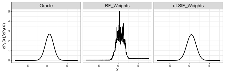
On data where $P_1$ and $P_2$ are known, compare a forest weighted by the true oracle ratio $dP_2^*/dP_1^*$ with one weighted by the uLSIF estimates across increasing shift strength, for example the Dirichlet simulation with $\lambda$ from 1 to 1.5. If the oracle-weighted forest tracks the $P_2$ generalization error while the estimated-weight forest diverges from it, the reweighting idea is sound and the fragility is in the weight estimator; if the oracle-weighted forest also fails, the covariate-shift assumption $P(Y\mid X)$ unchanged is the point of failure.
Extended reading notes
Core claim
Under the covariate-shift model $P_i(X,Y)=P(Y\mid X)P_i^*(X)$, the paper's central claim is that replacing the empirical node distribution inside a random forest with the weighted distribution $\tilde P_{A,w} = \sum_i w_i \mathbb{I}(X_i\in A)\delta_{(X_i,Y_i)} / \sum_j w_j \mathbb{I}(X_j\in A)$, where $w_i \propto \hat{\ell}(X_i)$ estimates $dP_2^*/dP_1^*$, makes both the split criterion $L(j,z)$ and the terminal-node prediction $T(x;D)$ approximate the target distribution $P_2$ instead of the training distribution $P_1$. The weights are learned from unlabeled test covariates, making the procedure semi-supervised. Proposition 1 states that the weighted out-of-bag error converges in probability to the $P_2$ generalization error, so tuning hyperparameters by minimizing weighted out-of-bag error selects a model for the target distribution. The paper also extends the weighting to quantile regression forests for prediction intervals and supplies a quantile-regression imputation step that preserves the training covariate distribution.
Load-bearing premise
The benefit of the method depends on the estimated weights being close to the true likelihood ratio $dP_2^*/dP_1^*$; Proposition 1 assumes the sup-norm estimation error tends to zero, but the paper does not verify this on the hurricane data and its simulations show the weighted forest's advantage erodes and can reverse as the shift grows.
Editorial extensions
If this is right
- Weighted out-of-bag error can be used to tune $mtry$ and other hyperparameters when the test distribution differs from training, without labeled test data (Proposition 1).
- The weighting extends to quantile regression forests, giving prediction intervals that stay near nominal coverage while growing narrower under covariate shift.
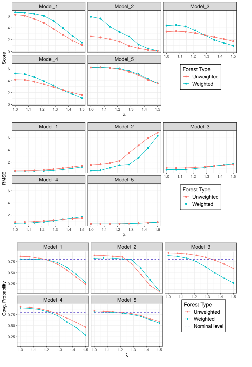
- In the simulations, the weighted forest improves RMSE and score over an unweighted forest for moderate shifts, with the largest gains in Models 1 and 2.
- Gains shrink as the shift grows: both weighted and unweighted forests degrade with increasing $\lambda$, and the weighted forest can underperform on large shifts.
- The quantile-regression imputation procedure generates missing covariates from the full conditional distribution, preserving the training covariate distribution so the density-ratio weights remain meaningful.
Reading between the lines
- Because the weighted node distribution is defined without assuming a particular splitter, the same two-stage recipe could be tested in gradient-boosted trees or other recursive ensemble methods, an extension the paper does not explore.
- A practical diagnostic would be to compare the effective sample size after uLSIF with the effective sample size of the oracle weights; when these diverge, the weight estimator is the fragile component rather than the forest.
- The proof of Proposition 1 assumes nonnegative responses and bounded fourth moments, so applying the method to zero-inflated or censored outage counts is a natural stress test.
- Weighted out-of-bag error could be paired with conformal prediction under covariate shift to produce calibrated intervals for extreme storms, a neighbouring development the paper does not develop.
Signed reviews
Editorial analysis
A structured set of objections, weighed in public.
Referee Report
Summary. The paper proposes a weighted random forest procedure for prediction under covariate shift. The method estimates the likelihood ratio dP2*/dP1* between the test and training covariate distributions using uLSIF (Kanamori et al., 2009), then uses these weights both in the split-selection criterion and in the prediction stage of each tree, with a weighted quantile regression forest variant for prediction intervals. To stabilize the weights, Section 3.2.3 replaces w(X) with w(X)^lambda so that the effective sample size equals a pre-specified n0, and Section 3.3 introduces a weighted out-of-bag error for model tuning. Proposition 1 claims that this weighted OOB error converges in probability to the P2 generalization error. The paper also proposes a quantile-regression-based missing-data imputation scheme. The method is evaluated on five synthetic data-generating models with varying shift severity, comparing weighted and unweighted forests, and on a hurricane power-outage forecasting application with six held-out storms.
Significance. If the claimed properties hold, the paper makes a practically useful contribution: it extends random forests to covariate shift with a relatively simple modification, and the hurricane outage application is a credible motivating problem. A notable strength is the design of the simulation in Section 4.1, which compares the learned uLSIF weights against oracle weights and thereby isolates the reweighting mechanism from density-ratio estimation error. The paper also provides a theoretical target, Proposition 1, for justifying weighted OOB model selection, and it makes concrete, falsifiable predictions about performance as a function of shift magnitude. However, the theoretical support as currently stated does not cover the regularized weights actually used in the experiments, and the empirical sections lack uncertainty quantification. With those issues addressed, the paper would be a solid contribution to the covariate-shift and random-forest literatures.
major comments (3)
- [Section 3.2.3, Section 3.3, Appendix B] Proposition 1 does not apply to the weighting scheme actually implemented and evaluated. The proposition assumes w_N(x)=c dP2*/dP1*(x)+epsilon_N(x), but Section 3.2.3 replaces the estimated weights with w(X_i)^lambda, choosing lambda so that the effective sample size equals n0=0.75n; Table 3 reports lambda values of 0.0084, 0.1305, and 0.3602, for which the weight vector is not proportional to the likelihood ratio. Consequently, the tuning rationale in Section 3.3 -- that minimizing the weighted OOB error should select a good model for P2 -- is not supported by Proposition 1 for the regularized estimator used in the simulations and the hurricane study. Please either extend the consistency result to ESS-regularized weights or explicitly restrict the claim to the un-regularized estimator.
- [Appendix B] The proof of Proposition 1 has gaps that need repair. The variance bound for S_{1,n} requires a boundedness or finite-moment condition on the likelihood ratio, e.g., sup_x dP2*/dP1*(x)<infinity or a finite second moment under P1; the displayed step bounding E_{P1}[L(X)(mB-Y)^4] by max(E_P[W^4], E_P[Z^4]) is not justified as written because the change of measure is not controlled. In addition, after arguing that S_{2,N} -> 0, the text concludes Var(S2,N) -> 1; the limit should be 0. These issues matter because Proposition 1 is the stated theoretical basis for using the weighted OOB error in model selection.
- [Section 4.3, Figure 4, Tables A2-A6] The simulation results are reported without any measure of variability. Figure 4 and Tables A2-A6 show only point estimates averaged over the 150 runs, so the reader cannot assess whether differences such as Model 1 at lambda=1.5 (weighted RMSE 1.214 vs unweighted 1.404) are meaningful. The same tables also show that the weighted forest loses its advantage at high shift levels in Models 3 and 4, e.g., Table A4 at lambda=1.357 and higher, and the coverage plots show weighted intervals falling below the 0.80 nominal level in that regime. Please add standard errors, intervals, or statistical comparisons, and discuss explicitly the range of shift magnitudes in which the method is beneficial.
minor comments (6)
- [Proposition 1, Section 3.3] The notation in Proposition 1 is inconsistent: it samples (X_i,Y_i)_{i=1}^{n+m} but then defines N, n, and m=sum Z_i without clearly relating n and m to N. Please clarify the sample-size notation.
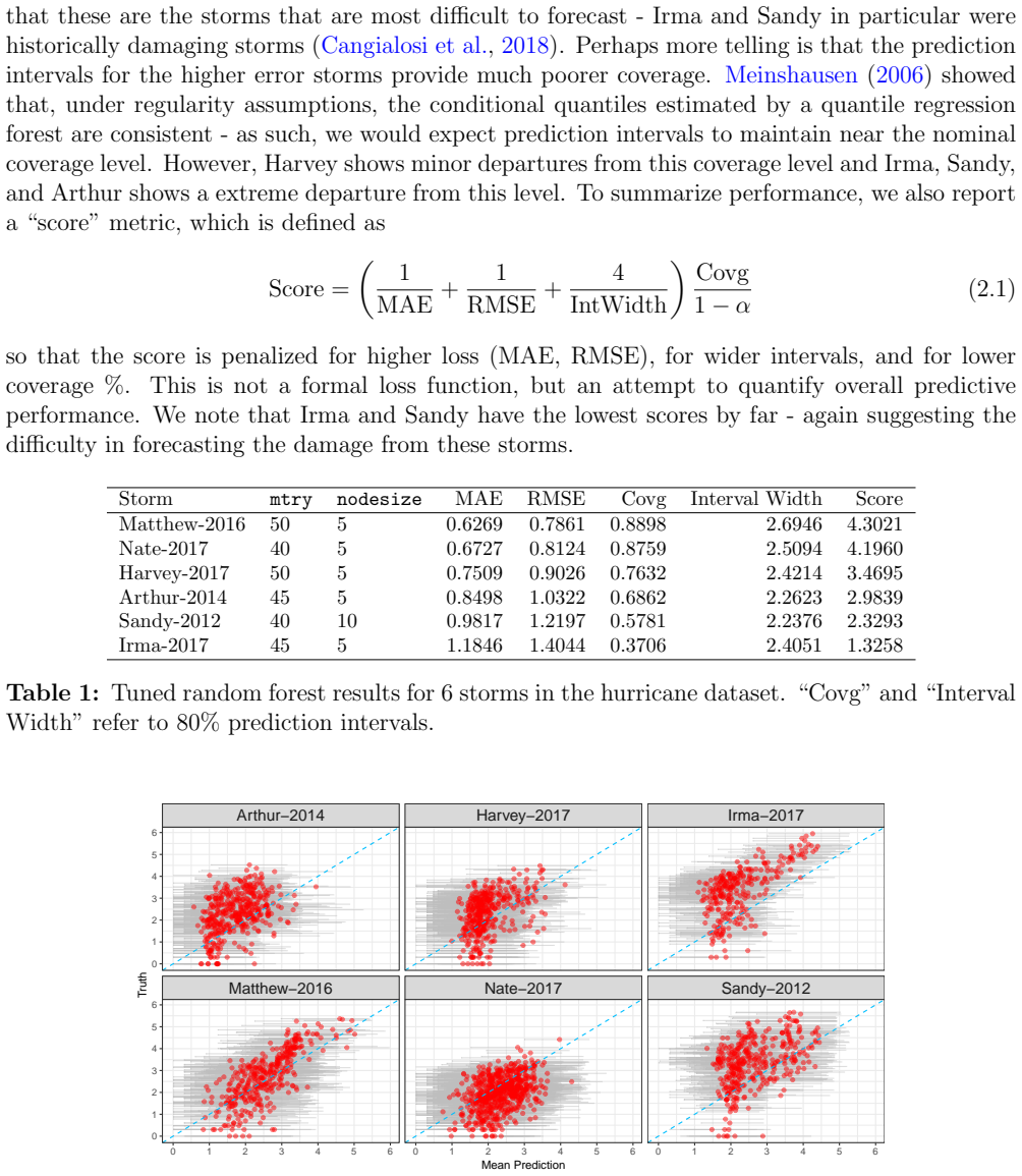
- [Section 5, Table 3] The hurricane results are mixed: the weighted model improves the score for Harvey, Irma, and Matthew, but for Sandy, Nate, and Arthur the weighted model is worse on most reported metrics, including score. The text should state this balance explicitly and discuss possible reasons, since the hurricane application is central to the paper's motivation.
- [Section 3.2.3] The statement that n0 is chosen in (1,n) conflicts with the later choice n0=0.75n; please specify whether n0 is an integer or a proportion and how the search for lambda is implemented.
- [Section 3.4, Equation (3.6)] Equation (3.6) is hard to parse: the displayed convergence appears to reverse the roles of the estimator and the limiting CDF. Rewriting this step would improve clarity.
- [Table 3] The lambda column is reported for unweighted rows as well as weighted rows; since unweighted forests do not use lambda, this is confusing and should be clarified in the table caption or by leaving those entries blank.
- [Figure 1 caption] The caption says "Fitted vs Predicted" but the figure appears to plot observed versus predicted values; please correct the wording.
Circularity Check
No significant circularity: the weighted OOB guarantee is a standard importance-sampling consistency result under an explicit weight-convergence hypothesis; the main caveats are unverified assumptions and proof gaps, not circular reasoning.
full rationale
Proposition 1 (Section 3.3, Appendix B) is the only candidate for a circular step, but on inspection it is not one. The weighted OOB metric in Eq. (3.5) is explicitly a self-normalized importance-sampling estimator, and its hypothesis w_N(x) = c dP2*/dP1* + epsilon_N(x) is an external consistency assumption about the uLSIF weight estimates, not a restatement of the conclusion theta_P2. The target theta_P2 is defined independently as the P2 expectation of the limiting OOB error, so the proposition's conclusion does not reduce to its input by construction; it is the standard importance-sampling identity, with a variance argument supplied in the proof. The proof does contain validity gaps — for example, the implemented ESS-regularized weights w(x)^lambda with lambda != 1 are not proportional to the likelihood ratio, so Proposition 1's hypothesis is not satisfied by the evaluated method, and the appendix contains an apparent slip in concluding Var(S2,N) -> 1 after showing S2,N -> 0. These are correctness and assumption gaps, not circularity. Likewise, the weights are estimated from unlabeled test covariates rather than test responses, and the simulations include oracle-weight comparisons that benchmark the weighting itself; the observed degradation under large shift (Figure 4, Section 6) is an empirical limitation, not a definitional identity. The self-citations (Mentch and Hooker; Coleman et al.; Peng et al.) appear only in related-work and simulation-design contexts and carry no load-bearing weight. No fitted parameter is renamed as a prediction, and no self-citation chain forces the paper's conclusions.
Assumptions & free parameters
free parameters (3)
- n0, minimum effective sample size target =
0.75n
- uLSIF bandwidth sigma =
not reported, selected by leave-one-out cross-validation
- uLSIF regularization parameter lambda =
not reported, selected by leave-one-out cross-validation
assumptions (6)
- domain assumption Covariate shift model: P1(X,Y)=P(Y|X)P1*(X) and P2(X,Y)=P(Y|X)P2*(X), so the conditional response distribution is identical across domains.
- domain assumption P1* and P2* are mutually absolutely continuous with matching support.
- ad hoc to paper Estimated weights are consistently proportional to the true likelihood ratio: wN(x)=c dP2*/dP1*(x)+epsilon_N(x) with sup|epsilon_N| -> 0.
- domain assumption Weak correlation of squared OOB residuals: rho*_n = max corr[(mB_i(X_i)-Y_i)^2, (mB_j(X_j)-Y_j)^2] -> 0.
- domain assumption Bounded fourth moments of Y and of tree predictions, with Y_i >= 0 almost surely.
- domain assumption Meinshausen quantile regression forests provide consistent conditional CDF estimators.
Cite this review
Pith. "Pith review of Locally Optimized Random Forests." pith.science (2026). https://pith.science/paper/7UK5ZU6T
@misc{pith2026190809967,
  author       = {Pith},
  title        = {Pith review of: Locally Optimized Random Forests},
  year         = {2026},
  howpublished = {\url{https://pith.science/paper/7UK5ZU6T}},
  note         = {Machine review of arXiv:1908.09967}
}
abstract
Standard supervised learning procedures are validated against a test set that is assumed to have come from the same distribution as the training data. However, in many problems, the test data may have come from a different distribution. We consider the case of having many labeled observations from one distribution, $P_1$, and making predictions at unlabeled points that come from $P_2$. We combine the high predictive accuracy of random forests (Breiman, 2001) with an importance sampling scheme, where the splits and predictions of the base-trees are done in a weighted manner, which we call Locally Optimized Random Forests. These weights correspond to a non-parametric estimate of the likelihood ratio between the training and test distributions. To estimate these ratios with an unlabeled test set, we make the covariate shift assumption, where the differences in distribution are only a function of the training distributions (Shimodaira, 2000.) This methodology is motivated by the problem of forecasting power outages during hurricanes. The extreme nature of the most devastating hurricanes means that typical validation set ups will overly favor less extreme storms. Our method provides a data-driven means of adapting a machine learning method to deal with extreme events.
Figures

Figures from the paper (2 more)

Reference graph
Works this paper leans on
-
[1]
Barber, R. F., Candes, E. J., Ramdas, A., and Tibshirani, R. J. (2019). Conformal prediction under covariate shift. arXiv preprint arXiv:1904.06019
arXiv 2019
-
[2]
Breiman, L. (2001). Random forests. Machine learning , 45(1):5--32
2001
-
[3]
Cangialosi, J. P., Latto, A. S., and Berg, R. (2018). Hurricane irma. In National Hurricane Center Tropical Cyclone Report
work page 2018
-
[4]
Chen, S. (2014). Imputation of missing values using quantile regression . PhD thesis, Iowa State University
work page 2014
-
[5]
Coleman, T., Peng, W., and Mentch, L. (2019). Scalable and efficient hypothesis testing with random forests. arXiv preprint arXiv:1904.07830
work page Pith review arXiv 2019
-
[6]
Friedman, J., Hastie, T., and Tibshirani, R. (2001). The elements of statistical learning , volume 1. Springer series in statistics New York, NY, USA:
work page 2001
-
[7]
Friedman, J. H. (1991). Multivariate adaptive regression splines. The annals of statistics , pages 1--67
work page 1991
-
[8]
Guikema, S. D. and Quiring, S. M. (2012). Hybrid data mining-regression for infrastructure risk assessment based on zero-inflated data. Reliability Engineering & System Safety , 99:178--182
work page 2012
Show all 32 references
-
[9]
W., Hartman, B
He, J., Wanik, D. W., Hartman, B. M., Anagnostou, E. N., Astitha, M., and Frediani, M. E. (2017). Nonparametric tree-based predictive modeling of storm outages on an electric distribution network. Risk Analysis , 37(3):441--458
2017
-
[10]
Kanamori, T., Hido, S., and Sugiyama, M. (2009). A least-squares approach to direct importance estimation. Journal of Machine Learning Research , 10(Jul):1391--1445
2009
-
[11]
Landsea , C. W. and Franklin , J. L. (2013). Atlantic Hurricane Database Uncertainty and Presentation of a New Database Format . Monthly Weather Review , 141:3576--3592
2013
-
[12]
A., Rosowsky, D
Liu, H., Davidson, R. A., Rosowsky, D. V., and Stedinger, J. R. (2005). Negative binomial regression of electric power outages in hurricanes. Journal of infrastructure systems , 11(4):258--267
2005
-
[13]
and Meng, X.-L
Liu, K. and Meng, X.-L. (2016). There is individualized treatment. why not individualized inference? Annual Review of Statistics and Its Application , 3:79--111
2016
-
[14]
Meinshausen, N. (2006). Quantile regression forests. Journal of Machine Learning Research , 7(Jun):983--999
2006
-
[15]
and Hooker, G
Mentch, L. and Hooker, G. (2016). Quantifying uncertainty in random forests via confidence intervals and hypothesis tests. The Journal of Machine Learning Research , 17(1):841--881
2016
-
[16]
and Hooker, G
Mentch, L. and Hooker, G. (2017). Formal hypothesis tests for additive structure in random forests. Journal of Computational and Graphical Statistics , 26(3):589--597
2017
-
[17]
Pasqualini, D., Kaufeld, K., and Dorn, M. F. (2017). Electric power outage forecasting model. Technical report, Los Alamos National Laboratory
2017
-
[18]
Peng, W., Coleman, T., and Mentch, L. (2019). Asymptotic distributions and rates of convergence for random forests and other resampled ensemble learners. arXiv preprint arXiv:1905.10651
2019 arXiv
-
[19]
Powers, S., Hastie, T., Tibshirani, R., et al. (2015). Customized training with an application to mass spectrometric imaging of cancer tissue. The Annals of Applied Statistics , 9(4):1709--1725
2015
-
[20]
J., Poczos, B., and Smola, A
Reddi, S. J., Poczos, B., and Smola, A. (2015). Doubly robust covariate shift correction. In Twenty-Ninth AAAI Conference on Artificial Intelligence
2015
-
[21]
Shimodaira, H. (2000). Improving predictive inference under covariate shift by weighting the log-likelihood function. Journal of statistical planning and inference , 90(2):227--244
2000
-
[22]
Stekhoven, D. J. and B \"u hlmann, P. (2011). Missforest—non-parametric missing value imputation for mixed-type data. Bioinformatics , 28(1):112--118
2011
-
[23]
Sugiyama, M., Krauledat, M., and M \ A z ller, K.-R. (2007). Covariate shift adaptation by importance weighted cross validation. Journal of Machine Learning Research , 8(May):985--1005
2007
-
[24]
and M \"u ller, K.-R
Sugiyama, M. and M \"u ller, K.-R. (2005). Input-dependent estimation of generalization error under covariate shift. Statistics & Decisions , 23(4/2005):249--279
2005
-
[25]
M., Atkinson, E
Therneau, T. M., Atkinson, E. J., et al. (1997). An introduction to recursive partitioning using the rpart routines
1997
-
[26]
Tokdar, S. T. and Kass, R. E. (2010). Importance sampling: a review. Wiley Interdisciplinary Reviews: Computational Statistics , 2(1):54--60
2010
-
[27]
and Athey, S
Wager, S. and Athey, S. (2017). Estimation and inference of heterogeneous treatment effects using random forests. Journal of the American Statistical Association
2017
-
[28]
Wager, S., Hastie, T., and Efron, B. (2014). Confidence intervals for random forests: The jackknife and the infinitesimal jackknife. The Journal of Machine Learning Research , 15(1):1625--1651
2014
-
[29]
Wanik, D., Anagnostou, E., Hartman, B., Frediani, M., and Astitha, M. (2015). Storm outage modeling for an electric distribution network in northeastern usa. Natural Hazards , 79(2):1359--1384
2015
-
[30]
E., Rappaport, E., and Marks, F
Willoughby, H. E., Rappaport, E., and Marks, F. (2007). Hurricane forecasting: The state of the art. Natural Hazards Review , 8(3):45--49
2007
-
[31]
Wright, M. N. and Ziegler, A. (2015). Ranger: a fast implementation of random forests for high dimensional data in c++ and r. arXiv preprint arXiv:1508.04409
2015 arXiv
-
[32]
Xu, R., Nettleton, D., and Nordman, D. J. (2016). Case-specific random forests. Journal of Computational and Graphical Statistics , 25(1):49--65
2016
Reviewed August 14, 2026 · model on record in the stance chip above.
Discussion (0). Continue with ORCID to comment.