REVIEW 2 major objections 4 minor 82 references
Stochastic order parameter dynamics for phase coexistence in heat conduction
T0 review · 2 major / 4 minor · reviewed 2026-08-14 · deepseek-v4-flash
Pith's one-line read A stochastic order-parameter model for phase coexistence in steady heat conduction predicts that the interface temperature deviates from the equilibrium transition temperature by a term proportional to the heat flux and the difference of…
desk verdict A serious paper with a new variational principle; the interface-temperature formula is the valuable conjecture, but the coefficient 1/3 rests on an admittedly phenomenological step, so treat (VI.40) as conditional until the interface contribution is derived. read the letter →
The pith
A machine-rendered reading of the paper's core claim, the machinery that carries it, and where it could break.
The reading
What carries the argument
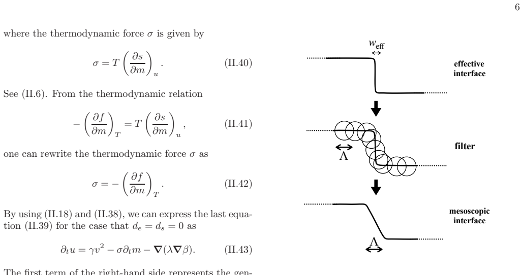
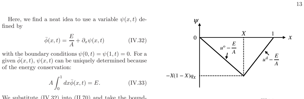
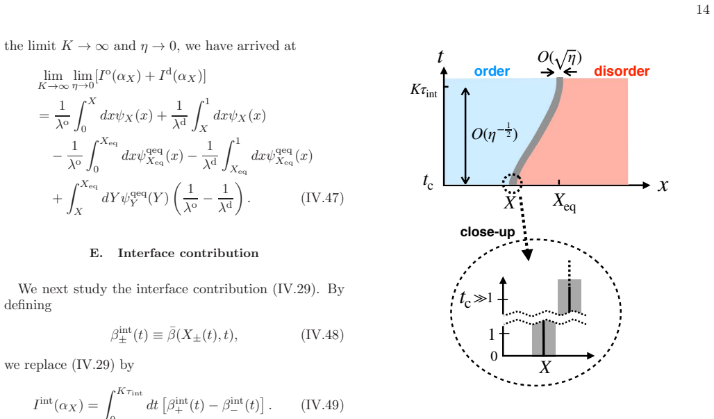
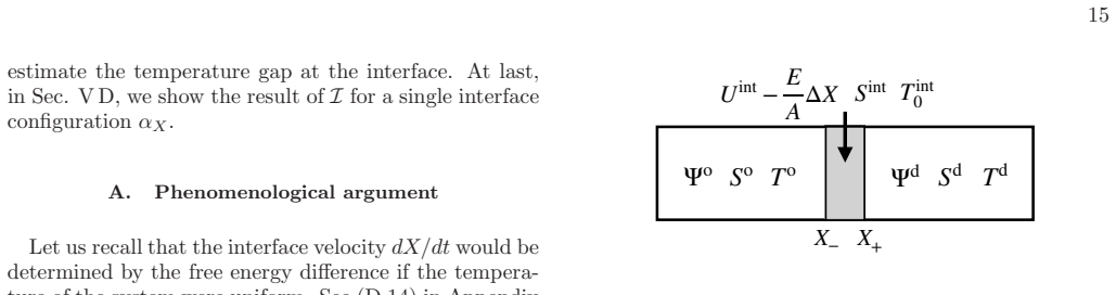
The central object is a stochastic extension of phase-field dynamics: fields $m$ (order parameter), $v$ (its momentum), and $\varphi$ (energy density), with an entropy functional $S=\int (s(u,m) - (d_s/2)|\nabla m|^2)$ and noise obeying local detailed balance; the small parameter $\eta$, the ratio of microscopic to system length, controls the separation of scales and makes interface motion singularly slow. The load-bearing identity is the stationary-distribution representation (the Zubarev\u2013McLennan form) $P_{ss}\propto e^{\tilde S/\eta^3}$, where the modified entropy $\tilde S = S + J I$ contains the time-integrated excess entropy production $I$ during relaxation of an interface configuration. The paper evaluates $I$ by splitting it into bulk and interface contributions; the interface contribution uses a phenomenological Onsager law for energy exchange between the interface and the two bulk regions with coefficients $L_o = \lambda_o/(g X_-)$ and $L_d = \lambda_d/(g(1-X_+))$, and the condition that the inverse-temperature gap vanish as the interface approaches either boundary fixes $g=1/3$. Maximizing $\tilde S$ over interface position $X$ produces the variational equation whose solution is the interface temperature formula.
What would settle it
A direct test is a numerical simulation of the stochastic model (II.65)\u2013(II.67) under the non-equilibrium adiabatic condition for a first-order order-disorder transition with unequal bulk conductivities: measure the steady interface temperature $\theta^*$ and check whether $\theta^*-T_c$ equals $-(J/3)(1/\kappa_o-1/\kappa_d)X_{eq}(1-X_{eq})$, in particular whether the deviation is linear in $J$, vanishes when $\kappa_o=\kappa_d$, and changes sign when the conductivity ordering is reversed. An independent check is a molecular-dynamics simulation of phase coexistence under a heat flux measuring the local temperature profile near the interface to see a superheated ordered or supercooled disordered layer of the predicted magnitude.
Extended reading notes
Core claim
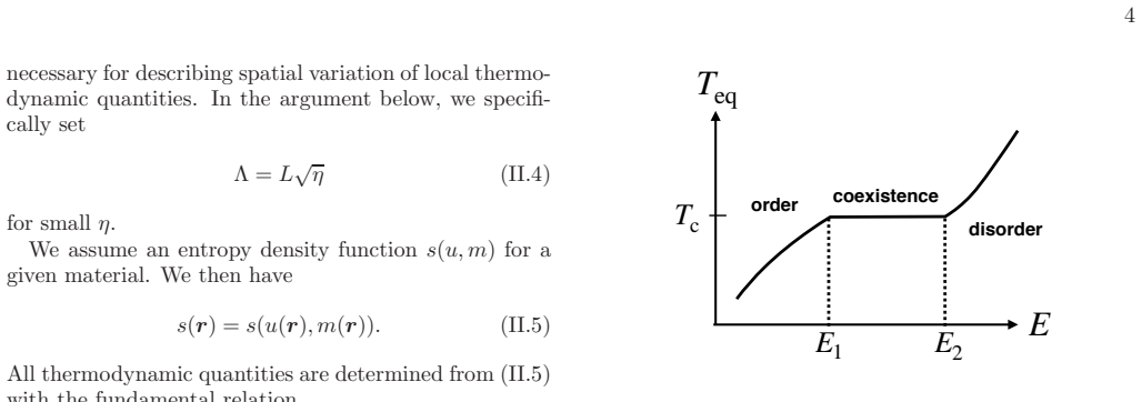
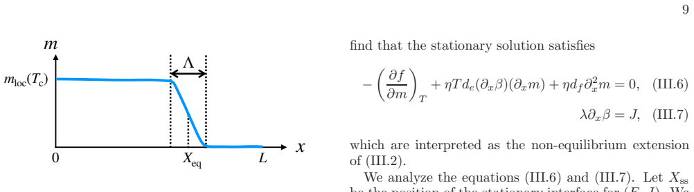
The central claim is that interface fluctuations, not deterministic bulk transport, set the coexistence temperature in steady heat conduction. The paper derives, within the linear response regime, the formula $\theta^* - T_c = -(J/3)(1/\kappa_o - 1/\kappa_d)X_{eq}(1-X_{eq})$, with $X_{eq}$ the equilibrium interface position, $\kappa_o$ and $\kappa_d$ the thermal conductivities of the ordered and disordered phases, and $J$ the heat flux ($J<0$ in the setup). Equivalently, for either sign of $J$, $\theta^* - T_c = |J|/3(1/\kappa_o - 1/\kappa_d)X_{eq}(1-X_{eq})$. The derivation proceeds by writing the stationary distribution of interface configurations through a modified entropy that includes the excess entropy produced during relaxation, decomposing that excess entropy into ordered-region, disordered-region, and interface parts, and maximizing the resulting potential over the interface position. The qualitative phenomenon\u2014superheated ordered or supercooled disordered states near the interface\u2014was predicted earlier by an extended thermodynamics framework; here it is obtained as the variational solution of a stochastic order parameter model, with a numerical prefactor $1/3$ instead of the earlier $1/2$.
Load-bearing premise
The load-bearing premise is that the energy exchange between the thin interface region and the two bulk regions is described by the phenomenological Onsager law (V.7)\u2013(V.10) with coefficients $L_o = \lambda_o/(g X_-)$ and $L_d = \lambda_d/(g(1-X_+))$, an uncontrolled approximation not yet derived from the stochastic model, and the factor $g=1/3$ is fixed by requiring the inverse-temperature gap to vanish at the boundaries.
Editorial extensions
If this is right
- For a first-order order\u2013disorder transition under steady heat flux, the coexistence line is not at $T_c$: the interface temperature shifts linearly with $J$, so measured phase diagrams in a thermal gradient should show a shifted apparent transition temperature at the interface.
- The sign of the shift is controlled by which phase conducts better: with the ordered phase less conductive, the ordered side is superheated; with the ordered phase more conductive, the disordered side is supercooled.
- The deviation vanishes when the two bulk conductivities are equal, so unequal conductivities are necessary for the effect; it also vanishes as the interface approaches either boundary, consistent with the boundary fixing of $g=1/3$.
- The deterministic, noiseless limit of the model predicts $\theta^*=T_c$, so the effect is carried by interface fluctuations: any coarse-grained description that omits the stochastic coupling of the interface to the bulk energy reservoirs would miss the shift.
- The variational potential $V(X)$ provides a way to compute other non-equilibrium thermodynamic properties of coexistence, such as the most probable interface position, once the stationary distribution of interface configurations is known.
Reading between the lines
- Because the authors conjecture the interface temperature is independent of the boundary condition for fixed energy and flux, the formula should also apply to the more standard setup of heat baths at the two ends; testing this in simulations would strengthen or falsify the conjecture.
- The numerical factor $1/3$, fixed by requiring the temperature gap to vanish at the boundaries, is likely the least secure part of the argument; a microscopic derivation of the Onsager coefficients $L_o,L_d$ from the stochastic model would either confirm $1/3$ or replace it, while the qualitative sign of the interface-temperature shift would probably survive.
- The same mechanism\u2014latent heat released by a fluctuating interface acting as a local heat source\u2014should appear in other first-order transitions such as liquid\u2013gas or nematic\u2013isotropic, with a conserved density adding an extra contribution; the paper mentions liquid\u2013gas as a natural next case.
- A direct numerical check of the stochastic model could measure the inverse-temperature gap during interface relaxation and compare it with the prediction $\beta_+^{int}-\beta_-^{int} = (1/3)(1/\lambda_o-1/\lambda_d)(dX/dt)X(1-X)q_X$, isolating the coefficient $1/3$.
Signed reviews
Editorial analysis
A structured set of objections, weighed in public.
Referee Report
Summary. The manuscript constructs a stochastic order-parameter model for a Z2 order-disorder transition coupled to heat conduction, and imposes a non-equilibrium adiabatic boundary condition in which the boundary energy flux is fixed while total energy is conserved. From the Zubarev-McLennan representation the authors derive a stationary distribution for single-interface configurations, decompose the excess entropy production into ordered-bulk, disordered-bulk, and interface contributions, and evaluate the bulk contributions from deterministic relaxation while estimating the interface contribution with a projected Onsager description. The resulting potential function V(X;E,J) leads to the main result (VI.40), θ*−Tc = −(J/3)(1/κ_o−1/κ_d) X_eq(1−X_eq), predicting a superheated ordered interface when κ_d>κ_o and a supercooled disordered interface when κ_d<κ_o, in qualitative agreement with the authors' earlier global thermodynamics.
Significance. The bulk calculation is clean and the variational structure is transparent; deriving a variational principle for phase coexistence under heat flow from a stochastic model would be a significant conceptual advance. The authors are explicitly honest about the weak point: in Sec. V A they state that Eqs. (V.7)–(V.10) "involve uncontrolled approximations" and are "not yet derived from the stochastic model." Because the entire numerical coefficient 1/3 in (VI.40) is fixed through this uncontrolled step and through the boundary-condition choice g=1/3, the paper at present establishes the qualitative sign of the effect but not the quantitative prediction. I regard this as a valuable framework whose headline claim needs either additional derivation or an explicit downgrading to a conjecture.
major comments (2)
- [Sec. V A, Eqs. (V.7)–(V.10), (V.52)–(V.54), and (VI.40)] The central quantitative result (VI.40) is carried by the interface contribution I_int, whose evaluation in Sec. V A rests on the phenomenological Onsager description (V.7)–(V.10) with diagonal coefficients L_o=λ_o/(g X_-) and L_d=λ_d/(g(1−X_+)). The authors themselves state that this description involves uncontrolled approximations and has not been derived from the stochastic model. The value g=1/3 is then imposed by requiring β_+^int−β_-^int to vanish as X→0 and X→1, not derived. If the true interface contribution differs (for example, if off-diagonal Onsager terms contribute, or if g depends on X), the coefficient multiplying J(1/κ_o−1/κ_d)X(1−X) changes: with no interface contribution it is 0, and the independent global-thermodynamics estimate is 1/2. Thus the numerical coefficient, which is the quantitative content of (VI.40), is not established. I recommend either deriving the interface contribution from the stochastic model or explicitly presenting (VI.40) as a qualitative/conjectural prediction and marking the 1/3 factor as a model-dependent estimate.
- [Sec. VI A, Eqs. (VI.1)–(VI.3)] The variational principle is introduced through the ansatz P(X;E,J)=exp([V(X;E,J)+O(√η)]/η^3) and the identification V(X;E,J)=max_{α_X∈C_X} \tilde S(α_X;E,J), which the authors describe only as a "reasonable conjecture." Since all subsequent equations in Sec. VI are manipulations of this V, the claim in the abstract that a variational principle is "derived" from the stochastic model goes beyond what is actually shown. This step should either be justified (at least to the same standard as the bulk contribution) or be stated explicitly as an unproved assumption of the framework.
minor comments (4)
- [Eq. (VI.32)] The definition f_d(θ_X)=u_o(θ_X)−θ_X s_d(θ_X) appears to contain a typo: the disordered free-energy density should use u_d(θ_X), not u_o(θ_X). As written, the combination f_o−f_d in (VI.37) and the subsequent derivation of (VI.38)–(VI.40) are confusing.
- [Caption of Fig. 1 and Sec. II E] The figure caption states J<0 while the text states J≤0. This is harmless but should be made consistent.
- [Sec. VI E] The sentence comparing the factor 1/3 with the factor 1/2 from global thermodynamics would be more useful with a specific equation reference to Ref. [17], so that readers can verify the comparison.
- [Author affiliation] There are minor typographical errors in the affiliation and email lines, e.g., "J apan" and "r nakayama@tohoku.ac.jp"; these should be corrected in the final version.
Circularity Check
No significant circularity: the central interface-temperature formula is derived from the stochastic model plus an explicitly phenomenological interface step, and the cited prior predictions are used only for comparison.
full rationale
The paper's central formula (VI.40) is not an input; it is the output of a chain that starts from the stochastic model (II.65)-(II.67), derives the Zubarev-McLennan stationary distribution (IV.7) and the modified entropy, computes the bulk excess-entropy-production terms (IV.47), and adds an interface term. The coefficient 1/3 enters through the phenomenological Onsager step (V.7)-(V.10): the parameter g is set to 1/3 by the boundary condition that the inverse-temperature gap vanish when the interface approaches the system boundaries (V.52)-(V.53). The authors explicitly state in Sec. V A that this description 'involves uncontrolled approximations' and is 'not yet derived from the stochastic model.' That is a serious limitation on the derivation's rigor and makes the quantitative coefficient conditional on a modeling assumption; it is not, however, circular, because the final temperature shift is not assumed at the outset, fitted to data, or obtained by renaming the prior thermodynamics result. The self-citations to the earlier prediction [16,17] are used for motivation and comparison ('If the factor 1/3 were 1/2, the result (VI.40) would be equivalent to the quantitative prediction by global thermodynamics'), not as the load-bearing derivation. Hence no circular step is present; the appropriate finding is score 0.
Assumptions & free parameters
free parameters (1)
- g =
1/3
assumptions (5)
- domain assumption A mesoscopic entropy functional S(m,u) = ∫ [s(u,m) - (d_s/2)|∇m|^2] with mean-field entropy density and no nucleation events.
- domain assumption The stochastic dynamics (II.65)-(II.67) with Gaussian white noise satisfying detailed balance and the non-equilibrium adiabatic boundary condition (II.73)-(II.74).
- domain assumption The stationary distribution has the Zubarev-McLennan form P_ss ∝ e^{S̃/η^3} with S̃ expanded to linear order in J.
- ad hoc to paper In the interface region the thermal conductivity λ is O(√η) and its functional form is not specified (IV.19)-(IV.20).
- ad hoc to paper The Onsager description of energy exchange between interface and bulk regions, equations (V.7)-(V.10), with diagonal coefficients only and L_o = λ_o/(g X_-), L_d = λ_d/(g(1-X_+)).
Cite this review
Pith. "Pith review of Stochastic order parameter dynamics for phase coexistence in heat conduction." pith.science (2026). https://pith.science/paper/7W3EIUUW
@misc{pith2026190803029,
  author       = {Pith},
  title        = {Pith review of: Stochastic order parameter dynamics for phase coexistence in heat conduction},
  year         = {2026},
  howpublished = {\url{https://pith.science/paper/7W3EIUUW}},
  note         = {Machine review of arXiv:1908.03029}
}
read the original abstract
We propose a stochastic order parameter equation for describing phase coexistence in steady heat conduction near equilibrium. By analyzing the stochastic dynamics with a non-equilibrium adiabatic boundary condition, where total energy is conserved over time, we derive a variational principle that determines thermodynamic properties in non-equilibrium steady states. The resulting variational principle indicates that the temperature of the interface between the ordered region and the disordered region becomes greater (less) than the equilibrium transition temperature in the linear response regime when the thermal conductivity in the ordered region is less (greater) than that in the disordered region. This means that a super-heated ordered (super-cooled disordered) state appears near the interface, which was predicted by an extended framework of thermodynamics proposed in [N. Nakagawa and S.-i. Sasa, Liquid-gas transitions in steady heat conduction, Phys. Rev. Lett. {\bf 119}, 260602, (2017).]
Figures

Figures from the paper (11 more)




Reference graph
Works this paper leans on
-
[1]
inverse-temperature gap
We also impose that the interface configuration satis- fies |¯v(x)| ≤ δv, (IV.18) where the constant δv is much smaller than 1. Since we consider the limit η → 0, the final result is independent of the parameters ( δm,δ v,r ). For a given single interface configuration αX , we study the time evolution from αX . We assume that a config- uration at any time t in...
-
[2]
Here, a1,a2,a3, and T0 are positive constants
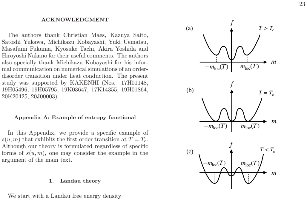
Landau theory We start with a Landau free energy density f (T,m ) = a1 2 (T −T0)m2 −a2 4 m4 +a3 6 m6 +ϕ(T ), (A.1) which describes the first order transition at some temper- atureTc. Here, a1,a2,a3, and T0 are positive constants. The functional form of ϕ(T ) will be determined later. See (A.16). For a given T , the equilibrium value meq(T ) ≥ 0 is determin...
-
[3]
E. Ben-Jacob and P. Garik, The formation of patterns in nonequilibrium growth, Nature 343, 523-530 (1990)
work page 1990
-
[4]
(A.13) 24 − m loc (T ) m loc (T ) m T T 1 T 0 m 1 T FIG
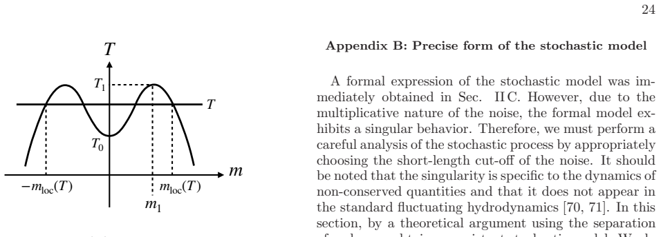
Entropy density The entropy density s(T,m ) is given by s = − ( ∂f ∂T ) m (A.12) = −a1 2 m2 −ϕ′(T ). (A.13) 24 − m loc (T ) m loc (T ) m T T 1 T 0 m 1 T FIG. 12. T (m) as a function of m. The internal energy density u(T,m ) is determined as u(T,m ) = −a1 2 T0m2 − a2 4 m4 + a3 6 m6 +ϕ(T ) −Tϕ ′(T ). (A.14) For simplicity, we assume that the heat capacity p...
work page 1970
-
[5]
Preliminaries for the derivation In order to derive the stochastic model, we rewrite the set of deterministic equations, (II.31), (II.32), and (II.33), as the simplest form. The key concept here is to introduce q by φ = E LLyLz + ∇q, (B.1) where we impose qn = 0 at the boundaries so as to satisfy (II.19). We express (B.1) as φ =φ(q). We here note S(m,v,φ ...
-
[6]
Derivation Since we assume the cut-off length in the noise, (B.12) becomes a non-local form with using a functional of χ as Lab(χ; r, r′) ≡ ∫ d3r′′Lab(χ(r′′), ∇χ(r′′)) ×δΛ c(r − r′′)δΛ c (r′ − r′′), (B.20) which is illustrated in Fig. 13. Further, since the On- sager coefficients Lab in (B.10) depend on χ, we have to consider multiplicative nature of the noi...
-
[7]
H. B. Callen, Thermodynamics and an Introduction to Thermostatistics, 2nd ed. (Wiley, New York, 1985)
work page 1985
-
[8]
J. R. Thome, Boiling in microchannels: a review of exper- iment and theory, Int. J. Heat and Fluid flow 25, 128-139 (2004)
work page 2004
Show all 82 references
-
[9]
D. M. Anderson, G. B. McFadden, and A. A. Wheeler, Diffuse-interface methods in fluid mechanics, Annual Re- view of Fluid Mechanics 30, 139-165 (1998)
1998
-
[10]
Ahlers, L
G. Ahlers, L. I. Berge, and D. S. Cannell, Thermal con- vection in the presence of a first-order phase change, Phys. Rev. Lett. 70, 2399 (1993)
1993
-
[11]
Zhong, D
J.-Q. Zhong, D. Funfschilling, and G. Ahlers, Enhanced heat transport by turbulent two-phase Rayleigh-Benard convection, Phys. Rev. Lett. 102, 124501 (2009)
2009
-
[12]
In order to seek the solutions, we consider a1T ′(m) = 2a2m − 4a3m3 = 0, (A.8) which gives m = 0 and m = ±m1 with m1 = √ a2 2a3 . (A.9) By setting T1 =T (m1) = T0 + a2 2 4a1a3 , (A.10) we find three locally stable states m = 0 and m = ±mloc(T ) when T0 ≤ T ≤ T1, where mloc(T ) ...
-
[13]
Weiss and G
S. Weiss and G. Ahlers, Nematic-isotropic phase transi- tion in turbulent thermal convection, J. Fluid Mech. 737, 308-328 (2013)
2013
-
[14]
M. E. Cates and J. Tailleur, Motility-Induced Phase Sep- aration, Annual Review of Condensed Matter Physics 6, 219-244 (2015)
2015
-
[15]
Urbana, D
P. Urbana, D. Schmoranzerb, P. Hanzelkaa, K. R. Sreeni- vasanc, and L. Skrbekb, Anomalous heat transport and condensation in convection of cryogenic helium, Proc. Nat. Acad. Sci. 110, 8036-8039 (2013)
2013
-
[16]
Bedeaux, E
D. Bedeaux, E. Johannessen, and A. Røsjorde, The nonequilibrium van der Waals square gradient model.(I). The model and its numerical solution, Physica A 330, 329-353 (2003)
2003
-
[17]
Onuki, Dynamic van der Waals theory, Phys
A. Onuki, Dynamic van der Waals theory, Phys. Rev. E 75, 036304 (2007)
2007
-
[18]
Schmitz, Fluctuations in nonequilibrium fluids, Physics Reports 171, 1-58 (1988)
R. Schmitz, Fluctuations in nonequilibrium fluids, Physics Reports 171, 1-58 (1988)
1988
-
[19]
Bertini, A
L. Bertini, A. De Sole, D. Gabrielli, G. Jona-Lasinio, a nd C. Landim, Macroscopic fluctuation theory, Rev. Mod. Phys. 87, 593 (2015)
2015
-
[20]
Forster, D
D. Forster, D. R. Nelson, and M. J. Stephen, Large- distance and long-time properties of a randomly stirred fluid, Phys. Rev. A 16, 732 (1977)
1977
-
[21]
Hohenberg and B
P.C. Hohenberg and B. I. Halperin, Theory of dynamic critical phenomena, Rev. Mod. Phys. 49 435-479 (1977)
1977
-
[22]
Nakagawa and S.-i
N. Nakagawa and S.-i. Sasa, Liquid-gas transitions in steady heat conduction, Phys. Rev. Lett. 119, 260602 (2017)
2017
-
[23]
Nakagawa and S.-i
N. Nakagawa and S.-i. Sasa, Global thermodynamics for heat conduction states, J. Stat. Phys. 177, 825-888 (2019)
2019
-
[24]
E. F. Gramsbergen, L. Longa, and W.H. de Jeu, Landau theory of the nematic-isotropic phase transition, Physics Report 135, 195-257 (1986)
1986
-
[25]
Sekimoto, Stochastic Energetics , Lect
K. Sekimoto, Stochastic Energetics , Lect. Notes Phys. 799 (Springer-Verlag, Berlin, 2010)
2010
-
[26]
Seifert, Stochastic thermodynamics, fluctuation th e- orems and molecular machines, Rep
U. Seifert, Stochastic thermodynamics, fluctuation th e- orems and molecular machines, Rep. Prog. Phys. 75, 126001 (2012)
2012
-
[27]
D. J. Evans, E. G. D. Cohen, G. P. Morriss, Probability of second law violations in shearing steady states, Phys. Rev. Lett. 71, 2401–2404 (1993)
1993
-
[28]
Gallavotti and E
G. Gallavotti and E. G. D. Cohen, Dynamical Ensem- bles in Nonequilibrium Statistical Mechanics, Phys. Rev. Lett. 74, 2694 (1995)
1995
-
[29]
Kurchan, Fluctuation theorem for stochastic dynam- ics, J
J. Kurchan, Fluctuation theorem for stochastic dynam- ics, J. Phys. A: Math. Gen. 31, 3719 (1998)
1998
-
[30]
J. L. Lebowitz and H. Spohn, A Gallavotti–Cohen-type symmetry in the large deviation functional for stochastic dynamics, J. Stat. Phys. 95, 333 (1999)
1999
-
[31]
Maes, The fluctuation theorem as a Gibbs property, J
C. Maes, The fluctuation theorem as a Gibbs property, J. Stat. Phys. 95, 367-392 (1999)
1999
-
[32]
G. E. Crooks, Entropy production fluctuation theorem and the nonequilibrium work relation for free energy dif- ferences, Phys. Rev. E 60, 2721 (1999)
1999
-
[33]
Jarzynski, Nonequilibrium equality for free energy dif- ferences, Phys
C. Jarzynski, Nonequilibrium equality for free energy dif- ferences, Phys. Rev. Lett. 78, 2690–2693 (1997)
1997
-
[34]
Sasa, Derivation of hydrodynamics from the Hamil - tonian description of particle systems, Phys
S.-i. Sasa, Derivation of hydrodynamics from the Hamil - tonian description of particle systems, Phys. Rev. Lett. 112, 100602 (2014)
2014
-
[35]
Sasa, Collective dynamics from stochastic therm o- dynamics, New Journal of Physics 17, 045024 (2015)
S.-i. Sasa, Collective dynamics from stochastic therm o- dynamics, New Journal of Physics 17, 045024 (2015)
2015
-
[36]
D. N. Zubarev, Nonequilibrium Statistical Thermody- namics, (Consultants Bureau, New York, 1974)
1974
-
[37]
J. A. Mclennan, Phys. Fluids 3, 493 (1960); Introduction to Non-equilibrium Statistical Mechanics (Prentice-Hall, 1988)
1960
-
[38]
T. S. Komatsu and N. Nakagawa, Expression for the stationary distribution in nonequilibrium steady states, Phys. Rev. Lett. 100, 030601 (2008)
2008
-
[39]
T. S. Komatsu, N. Nakagawa, S.-i. Sasa, and H. Tasaki Representation of nonequilibrium steady states in large mechanical systems, J. Stat. Phys. 134, 401-423 (2009)
2009
-
[40]
Maes and K
C. Maes and K. Netoˇ cn´ y, Rigorous meaning of McLennan ensembles, J. Math. Phys. 51, 015219 (2010)
2010
-
[41]
Fang and C
G. Fang and C. A. Ward, Temperature measured close to the interface of an evaporating liquid, Phys. Rev. E 59, 417-428 (1999)
1999
-
[42]
E. T. Jaynes, The minimum entropy production princi- 31 ple, Ann. Rev. Phys. Chem. 31, 579- 601 (1980)
1980
-
[43]
M. J. Klein and P. H. E. Meijer, Principle of minimum entropy production, Phys. Rev. 96, 250-255 (1954)
1954
-
[44]
Maes and K
C. Maes and K. Netoˇ cn´ y, Minimum entropy produc- tion principle from a dynamical fluctuation law, J. Math. Phys. 48, 053306 (2007)
2007
-
[45]
Derrida, Non-equilibrium steady states: fluctuatio ns and large deviations of the density and of the current, J
B. Derrida, Non-equilibrium steady states: fluctuatio ns and large deviations of the density and of the current, J. Stat. Mech. P07023 (2007)
2007
-
[46]
Nemoto and S.-i
T. Nemoto and S.-i. Sasa, Thermodynamic formula for the cumulant generating function of time-averaged cur- rent, Phys. Rev. E 84, 061113 (2011)
2011
-
[47]
J. L. Lebowitz, E. Presutti, H. Spohn, Microscopic Mod- els of Hydrodynamic Behavior, J. Stat. Phys. 51, 841 (1988)
1988
-
[48]
L. D. Landau and E. M. Lifshitz, Fluid Mechanics, (Perg- amon Press, Oxford 1959)
1959
-
[49]
B. I. Halperin, P.C. Hohenberg, and S. K. Ma, Renormal- ization group methods for critical dynamics I. Recursion relations and effects of energy conservation, Phys. Rev. B 10 139-153, (1974)
1974
-
[50]
Penrose and P
O. Penrose and P. C. Fife, Thermodynamically consis- tent models of phase-field type for the kinetic of phase transitions, Physica D 43, 44-62 (1990)
1990
-
[51]
Fujitani, Perturbation calculation for the density pro- file across the flat liquid-vapor interface in the steady heat-flow state, J
Y. Fujitani, Perturbation calculation for the density pro- file across the flat liquid-vapor interface in the steady heat-flow state, J. Phys. Soc. Jpn. 79, 074002 (2010)
2010
-
[52]
Fukuma and Y
M. Fukuma and Y. Sakatani, Entropic formulation of rel- ativistic continuum mechanics, Phys. Rev. E 84, 026315 (2011)
2011
-
[53]
R. M. Townsend and S. A. Rice, Molecular dynamics studies of the liquid-vapor interface of water, J. Chem. Phys. 94, 2207 (1991)
1991
-
[54]
D. G. Triezenberg and R. Zwanzig, Fluctuation theory of surface tension, Phys. Rev. Lett. 28 1183-1185 (1972)
1972
-
[55]
Weeks, Structure and thermodynamics of the liquid - vapor interface, J
J.D. Weeks, Structure and thermodynamics of the liquid - vapor interface, J. Chem. Phys. 67 3106 (1977)
1977
-
[56]
R. P. Feynman, R. B. Leighton, and M. Sands, The Feyn- manLectures on Physics , Vol. I (Addison-Wesley, Read- ing, Mas-sachusetts, 1963) Chap. 39-4
1963
-
[57]
E. H. Lieb, Some problems in statistical mechanics that I would like to see solved, Physica A 263, 491 (1999)
1999
-
[58]
Gruber and J
C. Gruber and J. Piasecki, Stationary motion of the adi- abaticpiston, Physica A 268, 412 (1999)
1999
-
[59]
Gruber and L
C. Gruber and L. Frachebourg, On the adiabatic proper- ties of a stochastic adiabatic wall: Evolution, stationary non-equilibrium, and equilibrium states, Physica A 272, 392 (1999)
1999
-
[60]
Hatano and S.-i
T. Hatano and S.-i. Sasa, Steady-state thermodynam- ics of Langevin systems, Phys. Rev. Lett. 86, 3463–3466 (2001)
2001
-
[61]
T. S. Komatsu, N. Nakagawa, S.-i. Sasa, and H. Tasaki, Steady-state thermodynamics for heat conduction: Mi- croscopic derivation, Phys. Rev. Lett. 100, 230602 (2008)
2008
-
[62]
Nakagawa, Work relation and the second law of ther- modynamics in nonequilibrium steady states, Phys
N. Nakagawa, Work relation and the second law of ther- modynamics in nonequilibrium steady states, Phys. Rev. E 85, 051115 (2012)
2012
-
[63]
Bertini, D
L. Bertini, D. Gabrielli, G. Jona-Lasinio, and C. Landi m, Clausius inequality and optimality of quasistatic trans- formations for nonequilibrium stationary states, Phys. Rev. Lett. 110, 020601 (2013)
2013
-
[64]
Maes and K
C. Maes and K. Netoˇ cn´ y, A nonequilibrium extension of the Clausius heat theorem, J. Stat. Phys. 154, 188-203 (2014)
2014
-
[65]
Chiba and N
Y. Chiba and N. Nakagawa, Numerical determination of entropy associated with excess heat in steady-state ther- modynamics, Phys. Rev. E 94, 022115 (2016)
2016
-
[66]
Keizer, Thermodynamics at nonequilibrium steady states, J
J. Keizer, Thermodynamics at nonequilibrium steady states, J. Chem. Phys. 69, 2609 (1978)
1978
-
[67]
B. C. Eu, Irreversible thermodynamics of fluids, Annals of Physics 140, 341-371 (1982)
1982
-
[68]
D. Jou, J. Casas-V´ azquez, and G. Lebon, Extended ir- reversible thermodynamics, Rep. Prog. Phys. 51, 1105- 1179 (1988)
1988
-
[69]
Oono and M
Y. Oono and M. Paniconi, Steady state thermodynamics, Prog. Theor. Phys. Suppl. 130, 29 (1998)
1998
-
[70]
Sasa and H
S.-i. Sasa and H. Tasaki, Steady state thermodynamics, J. Stat. Phys. 125, 125–224 (2006)
2006
-
[71]
Bertin, K
E. Bertin, K. Martens, O. Dauchot, and M. Droz, Inten- sive thermodynamic parameters in nonequilibrium sys- tems, Phys. Rev. E 75, 031120 (2007)
2007
-
[72]
Pradhan, R
P. Pradhan, R. Ramsperger, and U. Seifert, Approximate thermodynamic structure for driven lattice gases in con- tact, Phys. Rev. E 84, 041104 (2011)
2011
-
[73]
Dickman, Failure of steady-state thermodynamics in nonuniform driven lattice gases, Phys
R. Dickman, Failure of steady-state thermodynamics in nonuniform driven lattice gases, Phys. Rev. E 90, 062123 (2014)
2014
-
[74]
Røsjorde, D
A. Røsjorde, D. W. Fossmo, D. Bedeaux, S. Kjelstrup, and B. Hafskjold, Nonequilibrium molecular dynamics simulations of steady-state heat and mass transport in condensation: I. Local equilibrium, J. Coll. Int. Sci. 232, 178-185 (2000)
2000
-
[75]
Ogushi, S
F. Ogushi, S. Yukawa, and N. Ito, Asymmetric struc- ture of gas-liquid interface, J. Phys. Soc. Jpn. 75, 07301- (2006)
2006
-
[76]
D. N. Zubarev and V. G. Morozov, Statistical mechanics of nonlinear hydrodynamic fluctuations, Physica 120A, 411-467 (1983)
1983
-
[77]
V. G. Morozov, On the Langevin formalism for nonlinear and nonequilibrium hydrodynamic fluctuations, Physica 126A, 443-460 (1984)
1984
-
[78]
Graham and H
R. Graham and H. Haken, Fluctuations and stability of stationary non-equilibrium systems in detailed balance, Z. Phys. 245, 141-153 (1971)
1971
-
[79]
Zwanzig, Memory effects in irreversible thermody- namics, Phys
R. Zwanzig, Memory effects in irreversible thermody- namics, Phys. Rev. 124, 983-992 (1961)
1961
-
[80]
Itami and S.-i
M. Itami and S.-i. Sasa, Universal form of stochastic ev o- lution for slow variables in equilibrium systems, J. Stat. Phys. 167, 46-63 (2017)
2017
-
[81]
Nakano and S.-i
H. Nakano and S.-i. Sasa, Statistical mechanical expre s- sions of slip length, J. Stat. Phys. 176, 312-357 (2019)
2019
-
[82]
Pomeasu, Front motion, metastability and subcritic al bifurcations in hydrodynamics, Physica 23D, 3-11 (1986)
Y. Pomeasu, Front motion, metastability and subcritic al bifurcations in hydrodynamics, Physica 23D, 3-11 (1986)
1986
Reviewed August 14, 2026 · model on record in the stance chip above.
Discussion (0). Continue with ORCID to comment.