REVIEW 3 major objections 4 minor 25 references
Relaxation of hierarchy in higher-dimensional Starobinsky model
T0 review · 3 major / 4 minor · reviewed 2026-08-14 · deepseek-v4-flash
Pith's one-line read In higher-dimensional versions of the Starobinsky inflation model, the effects of extra R^m terms on n_s and r shrink as D=2n grows.
desk verdict New analytic result: in D=2n Starobinsky inflation the shifts from a λ R^m term shrink with n, so λ constraints relax; the result is real but sits on an assumed 4D reduction. read the letter →
The pith
A machine-rendered reading of the paper's core claim, the machinery that carries it, and where it could break.
The reading
What carries the argument
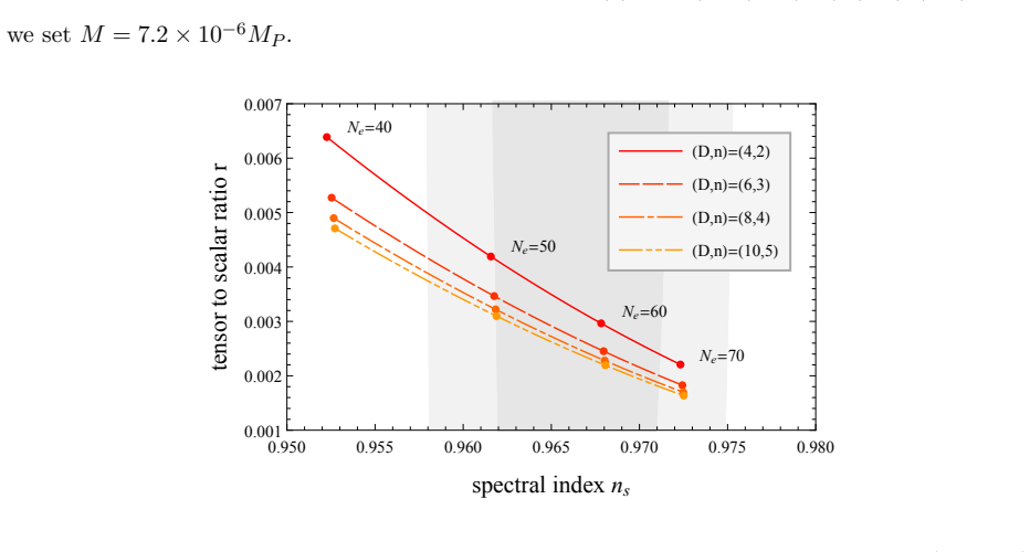
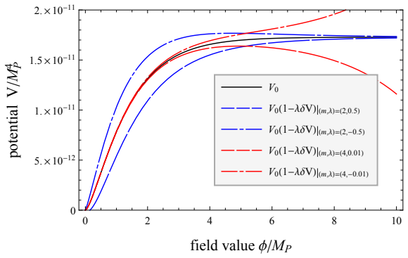
The load-bearing object is the dual Einstein-frame scalaron potential obtained from $F(R)$ gravity. The calculation is carried by a Legendre-Weyl transformation with an auxiliary field $\chi$, which turns $R+R^n/nM^{2n-2}+\lambda R^m/mM^{2m-2}$ into an Einstein-Hilbert term plus a canonical scalar field $\varphi$; the condition $D=2n$ makes the large-field potential flat, $V(\varphi)\propto(1-e^{-\alpha\varphi})^{n/(n-1)}$. The perturbation is then controlled by solving $(\chi/M^2)^{n-1}+\lambda(\chi/M^2)^{m-1}=e^{\alpha\varphi}-1$ by successive iteration and expanding the e-folding number with a Gauss hypergeometric function. What carries the suppression is the combination $(2n/(2n-1)N_e)^{(m-n)/(n-1)}$ in $\delta n_s$ and $\delta r$: with $N_e\sim 50$–$60$ and $m>n$, this factor is small, and it shrinks further as $n$ increases.
What would settle it
Solve Eq. (14) exactly, without the small-$\lambda$ iteration, for the $D=10$, $n=5$, $m=4$ case at $N_e=60$ and $\lambda$ near 0.3–0.5, where the paper reports the iterative method does not converge, and compute $n_s$ and $r$ directly; if these lie inside the current CMB-allowed region, the relaxation is even stronger than the paper claims, whereas if they lie outside, the wider $\lambda$ range is an artifact of the perturbative expansion.
Extended reading notes
Core claim
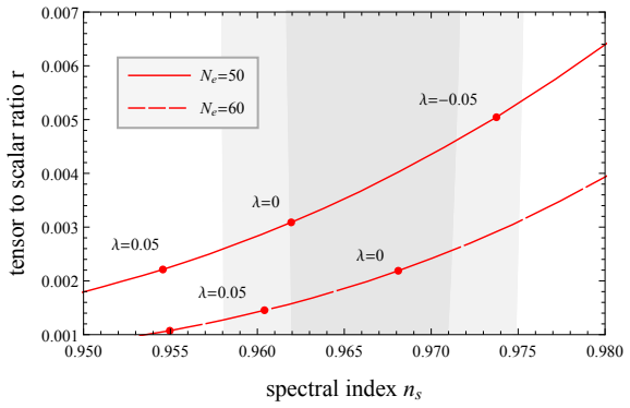
The paper's central claim is that in a $D=2n$ Starobinsky model with an added term $\lambda R^m/(mM^{2m-2})$, the leading shifts in the spectral index and tensor-to-scalar ratio are $\delta n_s = -\frac{4\lambda n(m-1)^2(m-n)}{m(n-1)^2(2n-1)(m+n-2)}\left(\frac{2n}{2n-1}N_e\right)^{\frac{m-n}{n-1}}$ and $\delta r = -\frac{32\lambda n^2(m-1)(m-n)}{m(n-1)^2(2n-1)(m+n-2)}\left(\frac{2n}{2n-1}N_e\right)^{\frac{m-n}{n-1}-1}$, up to higher order in slow-roll parameters. For $m>n$ the $N_e$-dependent factor is much smaller than one when $N_e\simeq 50$–$60$, and the prefactors fall roughly as $n^{-2}$, so the same value of $\lambda$ moves the predictions less as $D$ grows. Numerical evaluation in $D=10$ confirms the trend: the CMB-allowed range of $\lambda$ is orders of magnitude wider than in $D=4$ for the same $m$ and $N_e$. The paper concludes that the observational predictions of $D>4$ Starobinsky-like models are less sensitive to higher-curvature terms, which eases the hierarchy problem in constructing such models.
Load-bearing premise
The entire calculation assumes the higher-dimensional theory compactifies to a simple 4D action with only the scalaron kept, neglecting the dilaton and Kaluza-Klein vector and providing no stabilization of the extra dimensions; if compactification dynamics changes the effective potential, the predicted $\lambda$ sensitivity does not describe the higher-dimensional model.
Editorial extensions
If this is right
- For $D=2n$ models, each added $R^m$ term with $m>n$ moves $n_s$ and $r$ less than it would in 4D, so the observational predictions are more stable under unknown higher-curvature corrections.
- The CMB-allowed range of $\lambda$ becomes much wider in higher dimensions; in the paper's table, $D=10$ permits $\lambda$ values orders of magnitude above the $D=4$ bounds for the same $m$ and $N_e$.
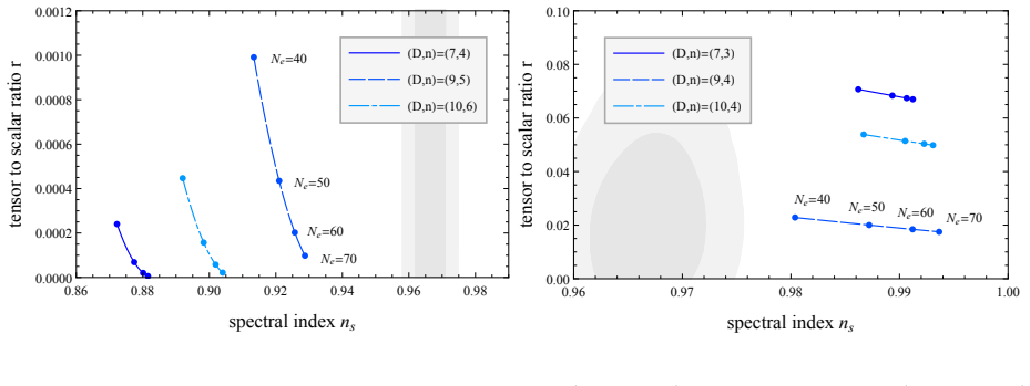
- Models with $D\neq 2n$ (for $4\le D\le 10$) are excluded by current CMB constraints, so the viable higher-dimensional branch is exactly the one whose predictions are robust to $R^m$ terms.
- Leading-order corrections from several $R^m$ terms add linearly, so terms with opposite signs of $\lambda_m(m-n)$ partially cancel, softening the hierarchy further.
- The leading-order tensor-to-scalar ratio $r = \frac{4(2n-1)}{(n-1)N_e^2}$ differs across dimensions, so future observations sensitive to $r$ could distinguish $D=4$ from $D>4$ models.
Reading between the lines
- If the suppression persists beyond first order, the same $N_e$-power mechanism should mute higher-curvature corrections to other observables such as the running of the spectral index, making the robust-prediction region of parameter space larger than the paper computes.
- The relaxation is established only where $\lambda$ is small enough for the successive-iteration method to converge; the $D=10$, $m=4$ case shows the method breaks down for larger $|\lambda|$, so an exact solution of Eq. (14) is the natural next test of whether the wider allowed range survives outside the perturbative regime.
- If a future measurement pins down $r$ at the level that distinguishes $D=4$ from $D=10$ at fixed $N_e$, it would indirectly probe the number of extra dimensions even when $\lambda$ is too small to be seen directly.
- A fundamental-theory embedding could use this result to identify the $R^2$ term as the leading higher-curvature correction, with other terms suppressed by volume or compactification effects rather than by a tuned hierarchy.
Signed reviews
Editorial analysis
A structured set of objections, weighed in public.
Referee Report
Summary. The paper studies a D-dimensional generalization of the Starobinsky model whose action contains R + R^n/nM^{2n-2} + λ R^m/mM^{2m-2}, with D=2n and m≠n. Working in the Einstein frame through the Legendre-Weyl transformation, the authors derive a 4D effective scalar potential under the explicit assumption that the dilaton and Kaluza-Klein vector are neglected and all fields depend only on 4D coordinates. For small λ they obtain analytic expressions for the potential, slow-roll parameters, and e-folding number, and from these they compute the leading shifts δn_s and δr in Eqs. (24)-(25). They find that for representative cases the shifts are suppressed by powers of N_e and by explicit 1/n^2 factors, so the Planck-allowed range of λ widens as D grows. Numerical integrations in §III.B, presented in Table I for D=4 and D=10, appear to corroborate this trend for several values of m. The paper also argues that D≠2n models are disfavored by Planck data and ends with a discussion of the remaining hierarchy between M and M_(D).
Significance. If the central claim is correct, the result is genuinely useful for higher-dimensional model building: it weakens a known fine-tuning problem of 4D Starobinsky inflation, namely the sensitivity of n_s and r to R^m corrections. The analytic formulas (24)-(25) are explicit and internally coherent, and the numerical scan provides a nontrivial check of the analytic approximation over a broad parameter range. The paper is also commendable for identifying and rejecting the D≠2n region, and for honestly flagging the schematic nature of the dimensional reduction. The main value is thus in establishing a scaling effect: higher-dimensional Starobinsky-like models are less sensitive to higher-curvature perturbations, provided the assumed 4D reduction is a valid description of the compactified theory.
major comments (3)
- [II.B, Eq. (9)] The entire calculation rests on the 4D action (9), which is assumed rather than derived from the D-dimensional dual action (8). The text states that the dilaton and Kaluza-Klein vector are neglected and that all fields depend only on 4D coordinates, but no stabilization mechanism for the extra dimensions is given, and no check is provided that the volume modulus (radion) and the scalaron remain canonically normalized and decoupled. Since Eqs. (17)-(25) and all numerical results are computed from this assumed potential, the paper establishes the relaxation of the λ bound only for the four-dimensional scalar-field model (9), not for the higher-dimensional theory announced in the title and abstract. I ask the authors to either supply a consistent truncation and stabilization analysis (or at least a concrete parametric regime where such a reduction is justified), or explicitly restate the central claim as a property of the assumed 4D effective action.
- [III.B, Table I] The allowed ranges for λ in Table I are obtained using only the 68% CL Planck constraint on n_s, together with the iterative-error criteria (28). The upper bound on r from Planck is not imposed, and the slow-roll truncation error is not propagated into the quoted intervals; several entries are labeled (PB), meaning no bound was obtained at all. These choices are not neutral for the claim that constraints are 'significantly relaxed' in higher dimensions: a more stringent r bound or a more complete treatment of slow-roll corrections could change the width and even the existence of the allowed intervals. Please quantify the sensitivity of the Table I bounds to these choices.
- [IV, Eq. (29)] The final compactification discussion asserts the bound M ≲ 1/V_extra^{1/(D-4)} and the scaling M ≲ O(10^{-5D/(2D-4)}) M_(D) without derivation. Combining M_P^2 = M_(D)^{D-2} V_extra with M_P ~ 10^5 M appears to produce a different exponent from Eq. (29) for D>4 (e.g., 10^{-10/(D-2)} rather than 10^{-5D/(2D-4)}), so the 'remaining hierarchy' statement is not yet settled. Please show the steps leading to Eq. (29) or correct it.
minor comments (4)
- [Throughout] There are several typographical and grammatical errors: 'Of cause' should be 'Of course', 'This result make' should be 'This result makes', 'mtirc' should be 'metric', and 'Here and χ is a solution' needs rewording.
- [Eq. (20)] The notation F(a,b,c,z) for the Gauss hypergeometric function is nonstandard; the usual notation is _2F_1(a,b;c;z). Please clarify the convention used.
- [Table I] The abbreviation (PB) is used for 'perturbation is broken', but the table renders it with a space as '(P B)'; please make the notation consistent and define it in the caption.
- [Figs. 5-7] In the captions of Figs. 5-7 it would help to state explicitly the values of (D,n) and m for each panel, as well as the meaning of the line color and style, since the current captions require the reader to infer these from the text.
Circularity Check
No significant circularity: the λ-shifts are derived from the assumed 4D action by standard f(R) duality and slow-roll analysis, then compared against external Planck data.
full rationale
The central derivation is self-contained. The action (12) with the extra λ R^m/mM^{2m−2} term is transformed into the dual scalar-tensor form (13) using the Legendre–Weyl procedure re-derived in Appendix A, and Eq. (14) is solved by successive iteration in λ to obtain the corrected potential (17). The slow-roll parameters (18)–(19), the e-folding expression (20), and its inversion (21) are then combined to produce the shifts δn_s and δr in Eqs. (24)–(25). No parameter is fitted to the Planck value of n_s: λ is a free input, and the allowed ranges in Table I are obtained by requiring the computed n_s and r to lie inside externally supplied Planck bounds. The base D=2n potential is not simply imported from the cited literature; the appendix re-derives the dual action for general F(R), and Eq. (10) follows by specialization. The main caveat, stated explicitly at Eq. (9): "we just assume the following 4-dimensional actions for simplicity ... we neglect dilaton and Kaluza-Klein vector," is a limitation about whether the assumed 4D action faithfully represents a stabilized compactification of the higher-dimensional theory. That is a completeness/correctness concern, not a circular reduction: the shifts are not defined in terms of the conclusion, nor is any fitted quantity renamed as a prediction. The final discussion of the remaining hierarchy via Eq. (29) is an auxiliary observation and does not enter the derivation of (24)–(25). Therefore the derivation chain is non-circular, and the appropriate score is 0.
Assumptions & free parameters
free parameters (1)
- M (higher-curvature mass scale) =
7.2e-6 M_P in the figures; otherwise left as a free model parameter
assumptions (4)
- domain assumption The higher-dimensional effective gravity action is the f(R) truncation Eq. (3), with only R, R^n and one λ R^m term relevant during inflation.
- ad hoc to paper The 4D potential Eq. (9) follows from assuming fields depend only on 4D coordinates and neglecting dilaton, Kaluza-Klein vector, and extra-dimensional stabilization dynamics.
- domain assumption The slow-roll approximation truncated at leading order in slow-roll parameters is valid, with N_e in the range 50 to 60.
- standard math The Legendre-Weyl transformation in Appendix A, including F''(χ) ≠ 0 and dropping total derivative terms, correctly dualizes f(R) gravity.
Cite this review
Pith. "Pith review of Relaxation of hierarchy in higher-dimensional Starobinsky model." pith.science (2026). https://pith.science/paper/A2AF3RSG
@misc{pith2026190809486,
  author       = {Pith},
  title        = {Pith review of: Relaxation of hierarchy in higher-dimensional Starobinsky model},
  year         = {2026},
  howpublished = {\url{https://pith.science/paper/A2AF3RSG}},
  note         = {Machine review of arXiv:1908.09486}
}
abstract
Starobinsky model, which has a Ricci scalar squared term $R^{2}$ in its action, is one of the most promising inflation models from the viewpoint of Cosmic Microwave Background observations. However, it is well known that observational predictions of this model are quite sensitive to the existence of $R^{m}$ $(2<m)$ terms, whose absence is just assumed. In this paper, we clarify that the observational predictions of $D$-dimensional ($4<D$) extended Starobinsky model are less sensitive to such terms than those of the original 4-dimensional model.This result make it easier to construct Starobinsky-like models in higher dimensions.
Figures

Figures from the paper (4 more)

Reference graph
Works this paper leans on
-
[1]
Although it is important to investigate the origin of the higher curv ature term for high energy physics, however, the origin is still unknown. One interestin g direction to unravel it is to regard such higher curvature term as a part of an effective act ion of high energy physics. For instance, a gravity part of string/M theory effective action is e xpecte...
-
[2]
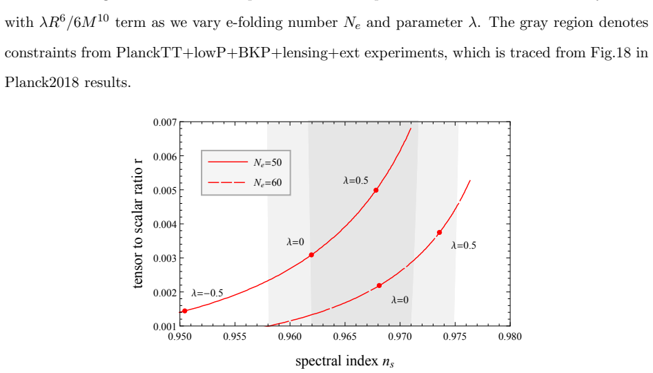
× 10-11 field value /MP potential V /MP4 FIG. 1. This figure shows the shapes of potentials of Eq.(9) wi th ( D, n ) = (6 , 2), (6, 3), (6, 4). Here we set M = 7. 2 × 10⁻⁶MP . Ne=40 Ne=50 Ne=60 Ne=70 (D,n)=(4,2) (D,n)=(6,3) (D,n)=(8,4) (D,n)=(10,5) 0.950 0.955 0.960 0.965 0.970 0.975 0.980 0.001 0.002 0.003 0.004 0.005 0.006 0.007 spectral index ns tensor ...
-
[3]
× 10-11 field value ϕ/MP potential V /MP4 FIG. 4. This figure shows the shape of potential Eq.(17) in ( D, n ) = (6 , 3) case, neglecting higher order terms O((λδV )2). Here we set M = 7. 2 × 10⁻⁶MP (λ < 0). The above statements can be confirmed explicitly by drawing the potential shape (Fig.4). From here on, we will discuss inflation using approximate poten...
-
[4]
A. A. Starobinsky, A New Type of Isotropic Cosmological M odels Without Singularity, Phys.Lett. B91 (1980)
work page 1980
-
[5]
A. D. Linde, A New Inflationary Universe Scenario: A Possi ble Solution of the Horizon, Flatness, Homogeneity, Isotropy and Primordial Monopole P roblems, Phys.Lett. 108B (1982) 389-393
work page 1982
-
[6]
A. Albrecht and P. J. Steinhardt, Cosmology for Grand Uni fied Theories with Radiatively Induced Symmetry Breaking, Phys.Rev.Lett. 48 (1982) 1220- 1223
work page 1982
-
[7]
Planck Collaboration (P. A. R. Ade et al.), Planck 2015 re sults. XX. Constraints on inflation, Astron.Astrophys. 594 (2016)Starobinsky’80 A20
work page 2016
-
[8]
Akrami et al.), Planck 2018 res ults
Planck Collaboration (Y. Akrami et al.), Planck 2018 res ults. X. Constraints on inflation, arXiv:1807.06211 [astro-ph.CO]
arXiv 2018
Show all 25 references
-
[9]
M. C. Bento and O. Bertolami, Maximally Symmetric Cosmol ogical Solutions of higher cur- vature string effective theories with dilatons, Phys.Lett. B 368 (1996) 198-201
1996
-
[10]
Lovelock, The Einstein tensor and its generalization s, J.Math.Phys
D. Lovelock, The Einstein tensor and its generalization s, J.Math.Phys. 12 (1971) 498-501
1971
-
[11]
Ostrogradsky, M´ emoires sur les ´ equations diff´ eren tielles, relatives au probl` eme des isop´ erim` etres, Mem.Acad.St.Petersbourg 6 (1850) no.4,385-517
M. Ostrogradsky, M´ emoires sur les ´ equations diff´ eren tielles, relatives au probl` eme des isop´ erim` etres, Mem.Acad.St.Petersbourg 6 (1850) no.4,385-517
-
[12]
Maeda, Towards the Einstein-Hilbert action via confo rmal transformation, Phys.Rev.D 39, 3159 (1989)
K. Maeda, Towards the Einstein-Hilbert action via confo rmal transformation, Phys.Rev.D 39, 3159 (1989)
1989
-
[13]
J. D. Barrow and S. Cotsakis, INFLATION AND THE CONFORMA L STRUCTURE OF HIGHER-ORDER GRA VITY THEORIES, Phys.Lett. B214, 4 (1988)
1988
-
[14]
Huang, A polynomial f(R) inflation model, JCAP 1402 (2 014) 035
Q. Huang, A polynomial f(R) inflation model, JCAP 1402 (2 014) 035
-
[15]
Asaka, S
T. Asaka, S. Iso, H. Kawai, K. Kohri, T. Noumi and T. Terad a, Reinterpretation of the Starobinsky model, PTEP 2016 (2016) no.12, 123E01
2016
-
[16]
S. V. Ketov and H. Nakada, Inflation from ( R + γR n − 2Λ) gravity in higher dimensions, Phys.Rev.D 95 103507 (2017)
2017
-
[17]
S. P. Otero, F. G. Pedro, and C. Wieck, R + αR n Inflation in higher-dimensional Space-times, JHEP 1705 (2017) 058 17
2017
-
[18]
S. V. Ketov and H. Nakada, Inflation from higher dimensio ns, Phys.Rev.D 96, 123530 (2017)
2017
-
[19]
Gunther, P
U. Gunther, P. Moniz and A. Zhuk, Asymptotical AdS from n onlinear gravitational models with stabilized extra dimensions, Phys.Rev. D66 (2002) 044 014 Erratum: Phys.Rev. D66 (2002) 089901
2002
-
[20]
Gunther, P
U. Gunther, P. Moniz and A. Zhuk, Nonlinear multidimens ional cosmological models with form fields: Stabilization of extra dimensions and the cosmologi cal constant problem, Phys.Rev. D68 (2003) 044010
2003
-
[21]
Gunther, A
U. Gunther, A. Zhuk, V. B. Bezerra and C. Romero, AdS and s tabilized extra dimensions in multidimensional gravitational models with nonlinear s calar curvature terms R−1 and R4, Class.Quant.Grav. 22 (2005) 3135-3167
2005
-
[22]
Kaneda, S
S. Kaneda, S. V. Ketov and N. Watanabe, Slow-roll inflati on in ( R + R4) gravity, Class.Quant.Grav. 27 (2010) 145016
2010
-
[23]
Motohashi, Consistency relation for Rp inflation, Phys.Rev
H. Motohashi, Consistency relation for Rp inflation, Phys.Rev. D91 (2015) 064016
2015
-
[24]
Boubekeur, D
L. Boubekeur, D. H. Lyth, Hilltop inflation, JCAP 0507 (2 005) 010
-
[25]
A. D. Felice and S. Tsujikawa, f(R) theories, arXiv:100 2.4928v2 [gr-qc] 18
Reviewed August 14, 2026 · model on record in the stance chip above.
Discussion (0). Continue with ORCID to comment.