Bregman Itoh--Abe methods for sparse optimisation

Carola-Bibiane Sch\"onlieb; Erlend S. Riis; Martin Benning

REVIEW 2 major objections 5 minor 61 references

Bregman Itoh--Abe methods for sparse optimisation

T0 review · 2 major / 5 minor · reviewed 2026-08-14 · deepseek-v4-flash

Challenge this review Re-run · record.json Download PDF Read on arXiv ↗ Review JSON

Pith's one-line read This paper proposes Bregman Itoh–Abe discrete-gradient methods for sparse optimisation and proves that, under its assumptions, all accumulation points of the amended scheme are Clarke stationary.

desk verdict Genuinely new Bregman discrete-gradient scheme with a clean dissipation structure, but the main stationarity theorem has an unproved monotonicity claim that the stress test exposes as a real gap. read the letter →

arxiv 1908.04583 v2 pith:A3SF6LXM submitted 2019-08-13 math.OC

Martin Benning , Erlend S. Riis , Carola-Bibiane Schönlieb This is my paper · ORCID

classification math.OC MSC 49M3749Q1565K1090C26

keywords BregmaniterationinversescalespaceflowdiscretegradientmethodsItoh–Abemethodnon-smoothoptimisationnon-convexsparseClarkestationarity

verification ladder T0 review T1 audit T2 compute T3 formal

The pith

A machine-rendered reading of the paper's core claim, the machinery that carries it, and where it could break.

The reading

The paper proposes optimisation methods for sparse variational-regularisation problems by discretising the inverse scale space flow with the Itoh–Abe discrete gradient. The resulting Bregman discrete-gradient schemes are unconditionally dissipative: the objective decreases for every choice of time step, with the decrease measured by a symmetric Bregman distance. The main theoretical claim is that, under Assumption 3.1, every accumulation point of the amended scheme is a Clarke stationary point of the objective restricted to a box constraint, even when the objective is non-smooth and non-convex. This matters because it provides convergence guarantees for a derivative-free, structure-preserving family of algorithms, and the numerical examples show sparse reconstructions obtained substantially faster than with plain SOR or Itoh–Abe methods.

What carries the argument

The central mechanism is the Bregman Itoh–Abe update, obtained by replacing the gradient in the coordinate-increment discrete gradient with the inverse-scale-space relation $p^{k+1}=p^k-\tau_k \bar\nabla V(x^k,x^{k+1})$. The Itoh–Abe discrete gradient is the coordinate-wise difference quotient (3.4); its mean-value property turns the decrease in $V$ into a symmetric Bregman distance, which by $\mu$-convexity of $J$ dominates $\|x^{k+1}-x^k\|^2$. The amendment (4.3) discards the part of the subgradient coming from the box constraint $\chi_{[l_i,u_i]}$, keeping the dual variables bounded when iterates sit on a bound.

What would settle it

Construct a locally Lipschitz, bounded-below objective on a box, together with a Bregman function meeting Assumption 3.1, where the amended scheme (4.3) has $V^o(x^k,e_i)<0$ at some iterate yet chooses $x^{k+1}_i < x^k_i$; or run the amended scheme on the Appendix A construction with the constraint subgradient forgotten and observe a subsequence stuck at $z=0$ while $\partial_z V = -1$. Either outcome would produce a limit point that is not Clarke stationary and would refute Theorem 4.5.

Watch

Extended reading notes

Core claim

The central claim is Theorem 4.5: for an objective $V$ and a Bregman function $J$ satisfying Assumption 3.1, all accumulation points of the amended Bregman Itoh–Abe scheme (4.3) are Clarke stationary points of $V$ restricted to the box $C$. The argument rests on the dissipation identity $V(x^k)-V(x^{k+1}) = \frac{1}{\tau_k} D^{\mathrm{symm}}_J(x^k,x^{k+1}) \ge \frac{\mu}{\tau_k}\|x^k-x^{k+1}\|^2$, which holds for arbitrary positive time steps. In a downhill coordinate direction the proof forces a long block of iterates to keep moving in that direction, so the corresponding dual variable $p_i$ would have to decrease without bound, contradicting boundedness of the coordinate subgradient of $J$ on a compact region. The amended scheme is necessary because the un-amended version can accumulate unbounded constraint subgradients and fail to converge to stationary points, as the appendix demonstrates.

Load-bearing premise

The proof depends on a monotonicity property it does not establish: whenever a coordinate direction is locally downhill, the implicit update is assumed to move that coordinate forward and never backward, and the box constraint is assumed to contribute nothing to the subgradient during that move.

Editorial extensions

If this is right

For any time-step sequence bounded between positive constants, the method is unconditionally dissipative: $V(x^{k+1}) \le V(x^k)$ and $\|x^{k+1}-x^k\| \to 0$, so the iterates settle rather than oscillate.
For non-smooth, non-convex objectives satisfying the assumptions, every accumulation point is Clarke stationary restricted to the box, extending the derivative-free Itoh–Abe guarantees to Bregman and inverse-scale-space discretisations.
For quadratic objectives the method reduces to SOR and coordinate descent when the Bregman function is the squared norm, and to a sparse SOR method when the Bregman function includes an $\ell^1$ term.
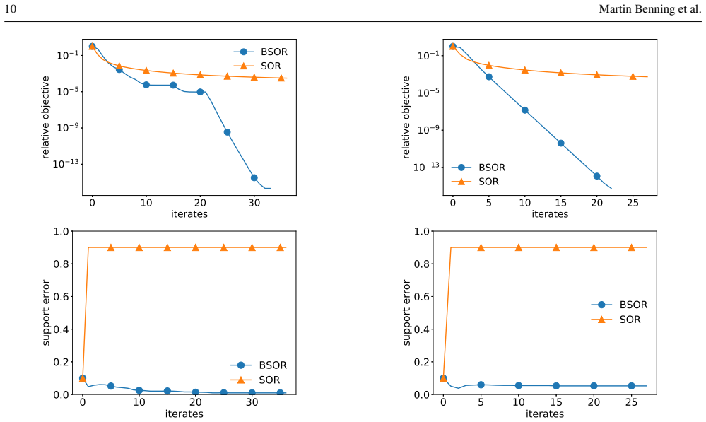
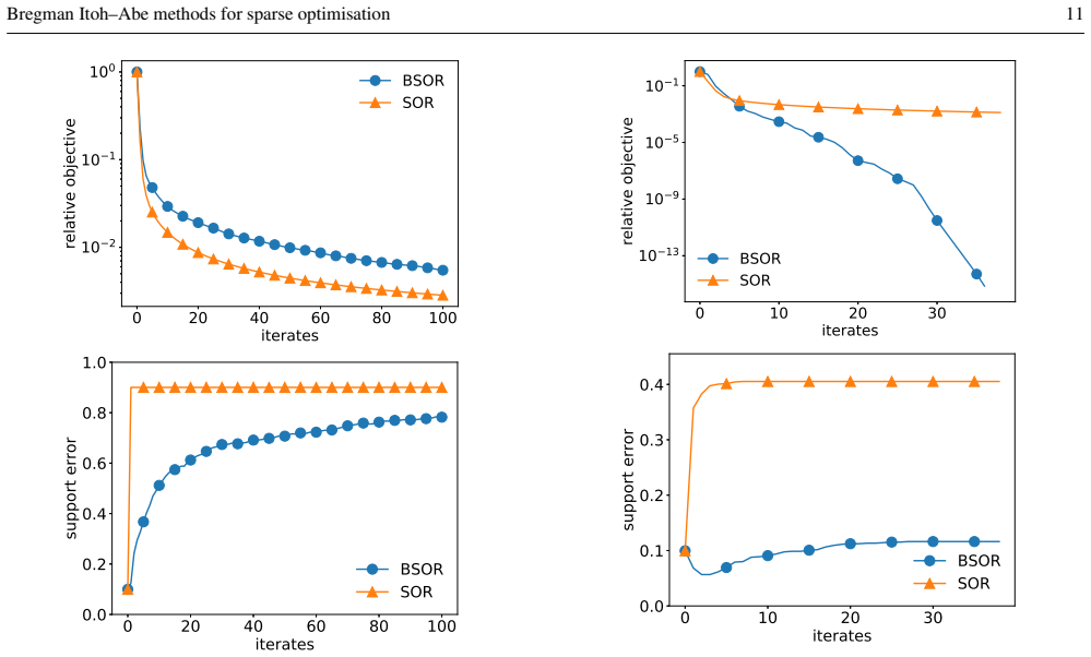
In the numerical examples, using a Bregman function that matches the sparsity of the problem substantially accelerates convergence in relative objective and support recovery compared with plain SOR and Itoh–Abe methods.
The un-amended scheme can fail, as the appendix shows, so forgetting the constraint subgradient is a necessary part of the convergence guarantee.

Reading between the lines

Editorial extensions of the paper, not claims the author makes directly.

Beyond the paper, the dissipation identity suggests a unified Lyapunov analysis: any discrete gradient satisfying the mean-value property, not only Itoh–Abe, could be inserted into the inverse-scale-space flow to obtain an unconditionally dissipative method.
The SOR and coordinate-descent equivalence indicates that Bregman discrete gradients could accelerate randomised coordinate descent for sparse least squares, a variant the paper does not test.
If the missing monotonicity of the implicit coordinate update is established, the same proof would likely transfer to local regularity classes such as prox-regular or lower-$C^2$ functions, since the uniqueness proposition already relies on local convexity bounds.
The imaging experiments exploit sparsity of the residual rather than the solution; a natural extension is transform-domain sparsity, where the Bregman function would be non-separable.

Share X Bluesky LinkedIn Reddit HN

Signed reviews

No signed human review yet.

Editorial analysis

A structured set of objections, weighed in public.

Desk editor's note, referee report, and a circularity audit.

Desk Editor's Note

read the letter

Two things to know up front. The core combination—discretizing the inverse scale space flow with Itoh–Abe discrete gradients—is genuinely new, and the dissipation structure is as clean as advertised. But the main convergence theorem has a real gap: the proof asserts monotone coordinate updates, and that assertion is not justified and can fail when the implicit update has multiple admissible roots.

What the paper does well. The dissipative identity (3.6) is correct and unconditional in the step size, which is the kind of structural guarantee discrete-gradient people care about. The well-posedness lemma is plausible and the amended scheme (4.3), which forgets constraint subgradients, comes with a real counterexample (Appendix A) showing the unmodified scheme can fail. That is honest and useful. The closed-form updates for sparse SOR variants are practical. The citation pattern is sound: the SOR equivalence is credited to Miyatake et al. and the convergence framework extends rather than borrows from Riis et al.

The soft spots. In the proof of Theorem 4.5, after assuming V^o(x*;ei) < -eta, the paper simply states that x^{k+1}_i >= x^k_i for the next N iterates and uses this to show the constraint subgradient vanishes and to bound the sum (4.5). Neither step is derived. The stress-test example is concrete and correct: with V(t) = -t + t^3 (suitably tail-extended), J = t^2/2, tau = 1, x = 0, p = 0, the equation y = -(V(y)-V(0))/y has roots y ≈ 0.618 and y ≈ -1.618, both satisfying the inclusion. So an admissible sequence can move left. Lemma 4.1 only guarantees existence of some y > x; it does not force the solution to be right-moving. Without a selection rule or a proof that all solutions move in the descent direction, the stationarity claim is not established for the method as written. Separately, Assumption 3.1(b) is not generally true for locally Lipschitz functions, yet the final inference from coordinate-wise conditions to Clarke stationarity on the box effectively relies on it. The theorem is therefore conditional on a structural property that is neither proven nor discussed.

Numbers and data. The experiments are illustrative: no error bars, no code, a few smallish problems. That is minor for this theory-first paper, but worth saying.

Bottom line. This is a valuable paper for people working on Bregman methods, geometric integration, and sparse inverse problems. It deserves a serious referee and, with a repaired stationarity proof, likely acceptance. The monotonicity gap is the thing to fix, not the overall direction.

Referee Report

2 major / 5 minor

Summary. This paper proposes a discrete-gradient discretisation of the inverse scale space flow, called the Bregman Itoh–Abe method, for constrained optimisation problems min_{x in C} V(x) with possibly non-convex, non-smooth V. The scheme (3.7)/(4.3) is shown to be unconditionally dissipative with respect to a symmetric Bregman distance (3.6); existence of updates is claimed in Lemma 4.1, uniqueness is proved under convexity or small-step weak convexity in Proposition 4.2, and Theorem 4.5 asserts that all accumulation points of the amended scheme are Clarke stationary under Assumption 3.1. The paper also derives closed-form sparse SOR variants, notes equivalences to SOR/coordinate descent for quadratic problems, and provides numerical experiments for sparse linear systems and a student-t regularised denoising problem.

Significance. The dissipative identity (3.6) is a clean and valuable contribution: it gives unconditional energy decay for arbitrary time steps and a natural Bregman generalisation of the Itoh–Abe discrete gradient. The closed-form BSOR updates and the numerical comparisons are useful and clearly presented. If Theorem 4.5 were fully established, the method would provide a derivative-free, dissipative scheme with Clarke-stationarity guarantees for a broad class of non-smooth, non-convex objectives. The paper also honestly includes a counterexample (Appendix A) showing why the unmodified scheme needs the amendment in (4.3). However, the proof of the main theorem has a load-bearing gap, and the final stationarity inference relies on a strong assumption whose role is not made explicit.

major comments (2)

[Section 4.3, proof of Theorem 4.5 (around (4.4)–(4.5))] The step 'since x^{k+1}_i >= x^k_i' is asserted without proof and is not a consequence of the scheme. Lemma 4.1 guarantees only existence of some solution of the implicit inclusion; Proposition 4.2 gives uniqueness only under convexity or small-step weak convexity, and neither is assumed in Theorem 4.5. In general (4.1) admits multiple admissible roots, including roots with y<x even when V^o(x;e_i)<0. For example, take V(t)=-t+t^3 extended by smooth quadratic tails so that V is bounded below and locally Lipschitz, J(t)=t^2/2, tau=1, x=0, p=0; the scalar inclusion p-(V(y)-V(0))/y in partial J(y) becomes y=1-y^2, whose roots are y about 0.618 and y about -1.618, both admissible. Thus an admissible sequence may move left, and the bound (4.5) does not follow for all sequences solving (4.3). The subsequent inference that the constraint component tilde q is zero is also not justified when an iterate is stationary at a lower bound, where partial chi_{[l_i,u_i]} is non-zero. The authors need either to impose a root-selection rule that guarantees the monotone root, or to prove the stationarity claim for every admissible root by a different argument.
[Section 4.3, final inference of Theorem 4.5] The proof establishes only the coordinate-wise inequalities V^o(x*;±e_i)>=0 (with the appropriate box sign), and then concludes Clarke stationarity. This conclusion is exactly Assumption 3.1(b), but that assumption is never cited or used in the proof. Assumption 3.1(b) is not a general property of locally Lipschitz functions: for V(x)=max{x_1,x_2}+(x_1+x_2)^2 at x=0, one has V^o(0;e_i)=1 and V^o(0;-e_i)=0 for i=1,2, while V^o(0;(-1,-1))=-1<0, so 0 is not Clarke stationary on C=R^2 although the coordinate-wise conditions hold. The theorem is therefore conditional on a nontrivial structural property, and the proof must either invoke (b) explicitly or replace it with a direct verification of stationarity on the tangent cone.

minor comments (5)

[Section 4.3, opening sentence] 'all accumulation points of the scheme (4.3) are nonstationary' should read 'stationary'; as printed it states the opposite of the theorem.
[Section 5.2, end of the paragraph after (5.5)] 'we leave include this in the appendix' is ungrammatical; it should be 'we leave this to the appendix'.
[Lemma 4.1 proof] The proof uses inequalities between sets, e.g. 'partial j(y) >= partial j(x)+mu(y-x)' and 'p-tau v^o(x;1) > partial j(y)'; since partial j(y) is an interval, these should be written for the relevant endpoints or in terms of support functions to be unambiguous.
[Assumption 3.1(b)] Assumption 3.1(b) deserves a remark: it is a genuine restriction (see Major Comment 2), and the paper should indicate where it is satisfied by the examples in Section 7.
[Section 7.1] The notation 'tau = 2/diag(A)' is a vector relation; the componentwise meaning should be stated explicitly, although (5.4) makes the intended interpretation clear.

Circularity Check

0 steps flagged · score 0.0 of 10

No significant circularity: the convergence theorem is proved from stated assumptions, and the self-citations to prior work are routine and not load-bearing.

full rationale

The central claim, Theorem 4.5, is derived in the paper from the dissipative identity (3.6), Lemma 4.1, Lemma 4.4, and the explicit assumptions in Assumption 3.1. No fitted parameter is renamed as a prediction, and no derived quantity is equal to an input by construction. Assumption 3.1(b) is an explicit structural condition on V and C; the theorem is conditional on it, so invoking it to pass from coordinate-wise directional inequalities to Clarke stationarity is a legitimate proof step, not a circular reduction. The citations to the authors' earlier work, especially [45] for the limit-set properties in Lemma 4.4(iii)-(iv), are self-citations, but those lemmas are auxiliary topological consequences and are not the source of the stationarity argument; the core dissipation and stationarity proof is carried out in this paper. The proof does contain an unproved assertion that x_i^{k+1} >= x_i^k in the proof of Theorem 4.5, and Assumption 3.1(b) may be too strong or not generally true, but these are correctness risks rather than cases where an output is equivalent to an input by definition or by self-citation. Accordingly, no specific circular step can be exhibited, and the appropriate finding is no significant circularity.

Assumptions & free parameters 3 free parameters · 4 assumptions · 0 invented entities

The central convergence result rests on Assumption 3.1, particularly the µ-convex separable form of J and box constraints. Assumption 3.1(b) appears superfluous and is questionable in general. The proof also rests on standard Clarke calculus and on the previous analysis of Itoh–Abe methods from [45], which the paper cites. No new entities are postulated.

free parameters (3)

time step τ (and coordinate scaling τ/diag(A)) = τ = 2/diag(A) or τ = 1 in examples
Algorithm step size chosen by hand for experiments; the theory allows any τ in [τmin, τmax], so it is not fitted to make the proof work.
Bregman sparsity parameter γ = γ = 1 (BSOR) or γ = 0.5 (denoising)
Trades off Euclidean vs l1 part in J(x) = 1/2||x||^2 + γ||x||_1; chosen by hand in numerical experiments.
regularisation parameter λ = λ = 100
Added to the objective V(x) = 1/2||Ax-b||^2 + λ||x||_1 in the noisy linear-system example; chosen by hand.

assumptions (4)

domain assumption Assumption 3.1(a): V is locally Lipschitz continuous and bounded below
Required for Clarke subdifferential framework and for the dissipation sum to converge; stated in Section 3.1.
domain assumption Assumption 3.1(c): constraint set C is a box
The coordinate-wise update structure of Itoh–Abe relies on separability of constraints; stated in Section 3.1.
domain assumption Assumption 3.1(d): J is proper, lsc, µ-convex with J(x) = Σ j_i(x_i) + χ_[l_i,u_i](x_i)
Ensures the Bregman distance bounds coordinate updates and that subdifferentials are separable; stated in Section 3.1.
ad hoc to paper Assumption 3.1(b): Clarke stationarity is equivalent to coordinate-wise directional derivative conditions
This equivalence is not generally true for arbitrary locally Lipschitz functions, and it is not used in the proof of Theorem 4.5, which establishes the more detailed boundary conditions directly.

how reviews work

0 comments

Cite this review

Pith. "Pith review of Bregman Itoh--Abe methods for sparse optimisation." pith.science (2026). https://pith.science/paper/A3SF6LXM

@misc{pith2026190804583,
  author       = {Pith},
  title        = {Pith review of: Bregman Itoh--Abe methods for sparse optimisation},
  year         = {2026},
  howpublished = {\url{https://pith.science/paper/A3SF6LXM}},
  note         = {Machine review of arXiv:1908.04583}
}

read the original abstract

In this paper we propose optimisation methods for variational regularisation problems based on discretising the inverse scale space flow with discrete gradient methods. Inverse scale space flow generalises gradient flows by incorporating a generalised Bregman distance as the underlying metric. Its discrete-time counterparts, Bregman iterations and linearised Bregman iterations, are popular regularisation schemes for inverse problems that incorporate a priori information without loss of contrast. Discrete gradient methods are tools from geometric numerical integration for preserving energy dissipation of dissipative differential systems. The resultant Bregman discrete gradient methods are unconditionally dissipative, and achieve rapid convergence rates by exploiting structures of the problem such as sparsity. Building on previous work on discrete gradients for non-smooth, non-convex optimisation, we prove convergence guarantees for these methods in a Clarke subdifferential framework. Numerical results for convex and non-convex examples are presented.

Figures

Figures reproduced from arXiv: 1908.04583 by the authors.

**Figure 7.2.** Comparison of SOR and sparse SOR methods, for Gaussian linear system without noise, and binary ground truth. Top: Convergence rate for relative objective. Bottom: Support error with respect to iterates. consider the simple case of finite difference approximations to first-order derivatives of x. We note that by applying a gradient flow to this regularisation function, we observe a similarity to Perona-Malik diffusio… view at source ↗

**Figure 7.4.** Comparison of SOR and sparse SOR methods, for ` 1 -regularised linear system with noise. Top: Convergence rate for relative objective. Bottom: Support error with respect to iterates. Appendix A Counterexample of Theorem 4.5 for (3.7) In the following example, we describe an example of a constrained optimisation problem for which the iterates of the unmodified Bregman Itoh–Abe method (3.7) fails to converge to a l… view at source ↗

**Figure 7.5.** Comparison of BIA and IA methods, for student-t regularised image denoising. First: Convergence rate for relative objective. Second: Convergence rate for relative gradient norm. Third: Input data. Fourth: Reconstruction. Next we define an objective function V : R 3 → R as folllows. Let fA, fB : R 2 → R be smooth support functions of A and B respectively, with disjoint support sets. That is, fA(x, y) ∈ [0,1], fB(x… view at source ↗

Discussion (0). Continue with ORCID to comment.

Reference graph

Works this paper leans on

61 extracted references · 56 canonical work pages

[1]

Lectures in Mathematics

Ambrosio, L., Gigli, N., Savare, G.: Gradient Flows: In Metric Spaces and in the Space of Probability Mea- sures, 2nd edn. Lectures in Mathematics. ETH Z ¨urich. Birkh¨auser Basel (2008)

work page 2008
[2]

Beck, A., Tetruashvili, L.: On the convergence of block coordinate descent type methods. SIAM J. Optim. 23(4), 2037–2060 (2013)

work page 2013
[3]

ArXiv e-prints (2017)

Benning, M., Betcke, M.M., Ehrhardt, M.J., Sch ¨onlieb, C.B.: Choose your path wisely: gradient descent in a Bregman distance framework. ArXiv e-prints (2017). URL http://arxiv.org/abs/1712.04045

arXiv 2017
[4]

Acta Numerica 27, 1–111 (2018)

Benning, M., Burger, M.: Modern regularization meth- ods for inverse problems. Acta Numerica 27, 1–111 (2018)

work page 2018
[5]

arXiv e-prints (2018)

Betancourt, M., Jordan, M.I., Wilson, A.C.: On sym- plectic optimization. arXiv e-prints (2018). URLhttp: //arxiv.org/abs/1802.03653

arXiv 2018
[6]

USSR Comput

Bregman, L.M.: The relaxation method of ﬁnding the common point of convex sets and its application to the solution of problems in convex programming. USSR Comput. Math. Math. Phys. 7(3), 200–217 (1967)

work page 1967
[7]

In: Advances in mathe- matical modeling, optimization and optimal control, pp

Burger, M.: Bregman distances in inverse problems and partial differential equations. In: Advances in mathe- matical modeling, optimization and optimal control, pp. 3–33. Springer (2016)

work page 2016
[8]

Burger, M., Gilboa, G., Moeller, M., Eckardt, L., Cremers, D.: Spectral decompositions using one- homogeneous functionals. SIAM J. Imag. Sci. 9(3), 1374–1408 (2016)

work page 2016

Show all 61 references

[9]

Burger, M., Gilboa, G., Osher, S., Xu, J.: Nonlinear in- verse scale space methods. Commun. Math. Sci. 4(1), 179–212 (2006)

2006
[10]

Burger, M., Moeller, M., Benning, M., Osher, S.: An adaptive inverse scale space method for compressed sensing. Math. Comput. 82(281), 269–299 (2013)

2013
[11]

Burger, M., Resmerita, E., He, L.: Error estimation for Bregman iterations and inverse scale space methods in image restoration. Comput. 81(2-3), 109–135 (2007)

2007
[12]

Cai, J.F., Osher, S., Shen, Z.: Linearized Bregman itera- tions for compressed sensing. Math. Comput. 78(267), 1515–1536 (2009)

2009
[13]

SIAM Journal on Scientiﬁc Computing 40(6), A3789–A3806 (2018)

Celledoni, E., Eidnes, S., Owren, B., Ringholm, T.: Dis- sipative numerical schemes on Riemannian manifolds with applications to gradient ﬂows. SIAM Journal on Scientiﬁc Computing 40(6), A3789–A3806 (2018)

2018
[14]

Censor, Y ., Zenios, S.A.: Proximal minimization algo- rithm with d-functions. J. Optim. Theory. Appl. 73(3), 451–464 (1992)

1992
[15]

Clarke, F.H.: Necessary conditions for nonsmooth prob- lems in optimal control and the calculus of variations. Ph.D. thesis, University of Washington (1973)

1973
[16]

Classics in Applied Mathematics

Clarke, F.H.: Optimization and Nonsmooth Analysis, 1st edn. Classics in Applied Mathematics. SIAM, Philadelphia (1990)

1990
[17]

Curry, H.B.: The method of steepest descent for non- linear minimization problems. Q. Appl. Math. 2(3), 258–261 (1944)

1944
[18]

Dong, B., Mao, Y ., Osher, S., Yin, W.: Fast linearized Bregman iteration for compressive sensing and sparse denoising. Commun. Math. Sci. 8(1), 93–111 (2010)

2010
[19]

Eckstein, J.: Nonlinear proximal point algorithms us- ing Bregman functions, with applications to convex pro- gramming. Math. Oper. Res. 18(1), 202–226 (1993)

1993
[20]

ArXiv e-prints (2018)

Eftekhari, A., Vandereycken, B., Vilmart, G., Zygalakis, K.C.: Explicit Stabilised Gradient Descent for Faster Strongly Convex Optimisation. ArXiv e-prints (2018). URL http://arxiv.org/abs/1805.07199

2018 arXiv
[21]

ArXiv e-prints (2018)

Ehrhardt, M.J., Riis, E.S., Ringholm, T., Sch ¨onlieb, C.B.: A geometric integration approach to smooth opti- misation: Foundations of the discrete gradient method. ArXiv e-prints (2018). URL http://arxiv.org/ abs/1805.06444

2018
[22]

SIAM, Philadelphia, PA, USA 14 Martin Benning et al

Ekeland, I., T ´eman, R.: Convex Analysis and Varia- tional Problems, 1st edn. SIAM, Philadelphia, PA, USA 14 Martin Benning et al. (1999)

1999
[23]

Gilboa, G., Moeller, M., Burger, M.: Nonlinear spectral analysis via one-homogeneous functionals: Overview and future prospects. J. Math. Imaging Vision 56(2), 300–319 (2016)

2016
[24]

Goldstein, T., Osher, S.: The split Bregman method for l1-regularized problems. SIAM J. Imag. Sci. 2(2), 323– 343 (2009)

2009
[25]

Gonzalez, O.: Time integration and discrete Hamilto- nian systems. J. Nonlinear Sci. 6(5), 449–467 (1996)

1996
[26]

Grimm, V ., McLachlan, R.I., McLaren, D.I., Quispel, G.R.W., Sch ¨onlieb, C.B.: Discrete gradient methods for solving variational image regularisation models. J. Phys. A 50(29), 295201 (2017)

2017
[27]

Hairer, E., Lubich, C.: Energy-diminishing integration of gradient systems. IMA J. Numer. Anal. 34(2), 452– 461 (2013)

2013
[28]

31, 2nd edn

Hairer, E., Lubich, C., Wanner, G.: Geometric numer- ical integration: structure-preserving algorithms for or- dinary differential equations, vol. 31, 2nd edn. Springer Science & Business Media, Berlin (2006)

2006
[29]

Neurocomputing 164, 45 – 55 (2015)

Hern ´andez-Solano, Y ., Atencia, M., Joya, G., Sandoval, F.: A discrete gradient method to enhance the numerical behaviour of Hopﬁeld networks. Neurocomputing 164, 45 – 55 (2015)

2015
[30]

Itoh, T., Abe, K.: Hamiltonian-conserving discrete canonical equations based on variational difference quotients. J. Comput. Phys. 76(1), 85–102 (1988)

1988
[31]

Springer Publishing Company, In- corporated, Berlin (2007)

Jahn, J.: Introduction to the Theory of Nonlinear Opti- mization, 3rd edn. Springer Publishing Company, In- corporated, Berlin (2007)

2007
[32]

Kiwiel, K.C.: Proximal minimization methods with generalized Bregman functions. SIAM J. Control Op- tim. 35(4), 1142–1168 (1997)

1997
[33]

Lorenz, D.A., Sch ¨opfer, F., Wenger, S.: The linearized Bregman method via split feasibility problems: analysis and generalizations. SIAM J. Imag. Sci. 7(2), 1237– 1262 (2014)

2014
[34]

arXiv e-prints (2014)

Lorenz, D.A., Wenger, S., Sch ¨opfer, F., Magnor, M.: A sparse Kaczmarz solver and a linearized Bregman method for online compressed sensing. arXiv e-prints (2014). URL http://arxiv.org/abs/1403.7543

2014 arXiv
[35]

arXiv e- prints (2018)

Maddison, C.J., Paulin, D., Teh, Y .W., O’Donoghue, B., Doucet, A.: Hamiltonian descent methods. arXiv e- prints (2018). URL http://arxiv.org/abs/1809. 05042

2018
[36]

McLachlan, R.I., Quispel, G.R.W.: Six lectures on the geometric integration of ODEs, p. 155–210. London Mathematical Society Lecture Note Series. Cambridge University Press, Cambridge (2001)

2001
[37]

McLachlan, R.I., Quispel, G.R.W., Robidoux, N.: Ge- ometric integration using discrete gradients. Philos. Trans. R. Soc. Lond. Ser. A Math. Phys. Eng. Sci. 357(1754), 1021–1045 (1999)

1999
[38]

Miyatake, Y ., Sogabe, T., Zhang, S.L.: On the equiv- alence between SOR-type methods for linear systems and the discrete gradient methods for gradient systems. J. Comput. Appl. Math. 342, 58–69 (2018)

2018
[39]

In: So- viet Mathematics Doklady, vol

Nesterov, Y .: A method of solving a convex program- ming problem with convergence rate O(1/k2). In: So- viet Mathematics Doklady, vol. 27, pp. 372–376 (1983)

1983
[40]

Ochs, P., Chen, Y ., Brox, T., Pock, T.: iPiano: Inertial proximal algorithm for nonconvex optimization. SIAM J. Imag. Sci. 7(2), 1388–1419 (2014)

2014
[41]

Multiscale Model

Osher, S., Burger, M., Goldfarb, D., Xu, J., Yin, W.: An iterative regularization method for total variation-based image restoration. Multiscale Model. Simul. 4(2), 460– 489 (2005)

2005
[42]

IEEE Trans

Perona, P., Malik, J.: Scale-space and edge detection using anisotropic diffusion. IEEE Trans. Pattern Anal. Mach. Intell. 12(7), 629–639 (1990)

1990
[43]

Poliquin, R., Rockafellar, R.: Prox-regular functions in variational analysis. Trans. Amer. Math. Soc. 348(5), 1805–1838 (1996)

1996
[44]

Quispel, G.R.W., Turner, G.S.: Discrete gradient meth- ods for solving ODEs numerically while preserving a ﬁrst integral. J. of Phys. A 29(13), 341–349 (1996)

1996
[45]

ArXiv e-prints (2018)

Riis, E.S., Ehrhardt, M.J., Quispel, G.R.W., Sch ¨onlieb, C.B.: A geometric integration approach to nonsmooth, nonconvex optimisation. ArXiv e-prints (2018). URL http://arxiv.org/abs/1807.07554

2018 arXiv
[46]

Ringholm, T., Lazi´c, J., Sch¨onlieb, C.B.: Variational im- age regularization with Euler’s elastica using a discrete gradient scheme. SIAM J. Imag. Sci. 11(4), 2665–2691 (2018)

2018
[47]

In: Annales de l’Institut Henri Poincare (C) Non Linear Analysis, vol

Rockafellar, R.: Maximal monotone relations and the second derivatives of nonsmooth functions. In: Annales de l’Institut Henri Poincare (C) Non Linear Analysis, vol. 2, pp. 167–184. Elsevier (1985)

1985
[48]

Princeton Landmarks in Mathematics and Physics

Rockafellar, R.T.: Convex analysis, 1st edn. Princeton Landmarks in Mathematics and Physics. Princeton uni- versity press, Princeton (2015)

2015
[49]

Santambrogio, F.:{Euclidean, metric, and Wasserstein} gradient ﬂows: an overview. Bull. Math. Sci. 7(1), 87– 154 (2017)

2017
[50]

In: International Conference on Scale-Space Theories in Computer Vision, pp

Scherzer, O., Groetsch, C.: Inverse scale space theory for inverse problems. In: International Conference on Scale-Space Theories in Computer Vision, pp. 317–
[51]

Inverse Problems 34(4), 179–212 (2018)

Schmidt, M.F., Benning, M., Sch ¨onlieb, C.B.: Inverse scale space decomposition. Inverse Problems 34(4), 179–212 (2018)

2018
[52]

Sch ¨opfer, F., Lorenz, D.A.: Linear convergence of the randomized sparse Kaczmarz method. Math. Program. 173(1), 509–536 (2019) Bregman Itoh–Abe methods for sparse optimisation 15

2019
[53]

In: Ad- vances in Neural Information Processing Systems, pp

Scieur, D., Roulet, V ., Bach, F., d’Aspremont, A.: Inte- gration methods and optimization algorithms. In: Ad- vances in Neural Information Processing Systems, pp. 1109–1118 (2017)

2017
[54]

Su, W., Boyd, S., Candes, E.J.: A differential equation for modeling Nesterov’s accelerated gradient method: theory and insights. J. Mach. Learn. Res. 17(153), 1–43 (2016)

2016
[55]

Teboulle, M.: Entropic proximal mappings with appli- cations to nonlinear programming. Math. Oper. Res. 17(3), 670–690 (1992)

1992
[56]

Proceedings of the National Academy of Sciences 113(47), E7351–E7358 (2016)

Wibisono, A., Wilson, A.C., Jordan, M.I.: A varia- tional perspective on accelerated methods in optimiza- tion. Proceedings of the National Academy of Sciences 113(47), E7351–E7358 (2016)

2016
[57]

arXiv e-prints (2016)

Wilson, A.C., Recht, B., Jordan, M.I.: A Lyapunov Analysis of Momentum Methods in Optimization. arXiv e-prints (2016). URL http://arxiv.org/abs/ 1611.02635

2016 arXiv
[58]

Mathe- matical Programming 1(151), 3–34 (2015)

Wright, S.J.: Coordinate descent algorithms. Mathe- matical Programming 1(151), 3–34 (2015)

2015
[59]

Yin, W., Osher, S., Goldfarb, D., Darbon, J.: Bregman iterative algorithms for 𝓁1-minimization with applica- tions to compressed sensing. SIAM J. Imag. Sci. 1(1), 143–168 (2008)

2008
[60]

Computer science and applied mathe- matics

Young, D.M.: Iterative Solution of Large Linear Sys- tems, 1st edn. Computer science and applied mathe- matics. Academic Press, Inc., Orlando, Florida (1971)

1971
[61]

Zhang, X., Burger, M., Osher, S.: A uniﬁed primal-dual algorithm framework based on Bregman iteration. J. Sci. Comput. 46(1), 20–46 (2011)

2011

Pith tools

Reviewed August 14, 2026 · model on record in the stance chip above.

[1] [1]

Lectures in Mathematics

Ambrosio, L., Gigli, N., Savare, G.: Gradient Flows: In Metric Spaces and in the Space of Probability Mea- sures, 2nd edn. Lectures in Mathematics. ETH Z ¨urich. Birkh¨auser Basel (2008)

work page 2008

[2] [2]

Beck, A., Tetruashvili, L.: On the convergence of block coordinate descent type methods. SIAM J. Optim. 23(4), 2037–2060 (2013)

work page 2013

[3] [3]

ArXiv e-prints (2017)

Benning, M., Betcke, M.M., Ehrhardt, M.J., Sch ¨onlieb, C.B.: Choose your path wisely: gradient descent in a Bregman distance framework. ArXiv e-prints (2017). URL http://arxiv.org/abs/1712.04045

arXiv 2017

[4] [4]

Acta Numerica 27, 1–111 (2018)

Benning, M., Burger, M.: Modern regularization meth- ods for inverse problems. Acta Numerica 27, 1–111 (2018)

work page 2018

[5] [5]

arXiv e-prints (2018)

Betancourt, M., Jordan, M.I., Wilson, A.C.: On sym- plectic optimization. arXiv e-prints (2018). URLhttp: //arxiv.org/abs/1802.03653

arXiv 2018

[6] [6]

USSR Comput

Bregman, L.M.: The relaxation method of ﬁnding the common point of convex sets and its application to the solution of problems in convex programming. USSR Comput. Math. Math. Phys. 7(3), 200–217 (1967)

work page 1967

[7] [7]

In: Advances in mathe- matical modeling, optimization and optimal control, pp

Burger, M.: Bregman distances in inverse problems and partial differential equations. In: Advances in mathe- matical modeling, optimization and optimal control, pp. 3–33. Springer (2016)

work page 2016

[8] [8]

Burger, M., Gilboa, G., Moeller, M., Eckardt, L., Cremers, D.: Spectral decompositions using one- homogeneous functionals. SIAM J. Imag. Sci. 9(3), 1374–1408 (2016)

work page 2016