REVIEW 5 major objections 5 minor 35 references
Quick-Draw Bandits: Quickly Optimizing in Nonstationary Environments with Extremely Many Arms
T0 review · 5 major / 5 minor · reviewed 2026-08-07 · deepseek-v4-flash
Pith's one-line read The Quick-Draw bandit policy models rewards as Gaussian interpolations over space and time and claims $\mathcal{O}^*(\sqrt{T})$ cumulative regret on Lipschitz reward functions, with an extension to nonstationary environments and a large…
desk verdict The algorithm is fast and the experiments are strong, but the advertised O*(sqrt T) regret bound is not proven: the bandwidth condition makes the constant horizon-dependent and the proof contains a reversed inequality, so the theory does not support the claim. read the letter →
The pith
A machine-rendered reading of the paper's core claim, the machinery that carries it, and where it could break.
The reading
What carries the argument
The central object is the Quick-Draw index. For each arm $x$ at round $T$ it computes $\hat\Sigma_T(x)=\left(\sum_{s=1}^T 1/\hat\sigma_s^2(x)\right)^{-1/2}$ and $\hat\mu_T(x)=\hat\Sigma_T^2(x)\sum_{s=1}^T y_s/\hat\sigma_s^2(x)$, which are the standard deviation and mean of the product of $T$ Gaussian likelihoods; the index is $\mathrm{UCB}=\min(\hat\mu_T+\gamma_{T+1}\hat\Sigma_T,1)$, with $\gamma_{T+1}$ set by a concentration bound. The $\hat\sigma_s^2$ term encodes the Lipschitz assumption in space and time: uncertainty grows quadratically with distance from observed arms, so nearby observations are weighted more heavily. The proof carries the argument through a martingale concentration inequality on the weighted observation errors and a Cauchy--Schwarz bound on the Lipschitz bias, with the bandwidth $\ell_x$ controlling the uniform concentration (Theorem 4.1).
What would settle it
Run Quick-Draw on a known one-dimensional Lipschitz reward, e.g., $\mu(x)=x$ on $[0,1]$, with the paper's default parameters ($\ell_x=\ell_t=1$, $\rho^2=10^{-7}$) and measure cumulative regret at $T=10^3,10^4,10^5,10^6$. If the regret at the horizon grows faster than $\sqrt{T}$, the claimed $\mathcal{O}^*(\sqrt{T})$ rate does not hold in the regime the paper evaluates. A simpler check: confirm whether the experimental configuration ($T_{\max}=1000$, $\ell_x=1$) satisfies $\ell_x \le 1/\sqrt{T_{\max}-\rho^2}$ (it does not), which would mean the reported empirical results lie outside the theorem's assumptions.
Extended reading notes
Core claim
The central claim is that a simple product-of-Gaussians estimator---each past observation contributes a Gaussian likelihood with variance $\hat\sigma_s^2(x,t)=\rho^2+(D(x,x_s)/\ell_x)^2+((t-t_s)/\ell_t)^2$---produces a closed-form posterior mean $\hat\mu_T(x)$ and standard deviation $\hat\Sigma_T(x)$ that can drive a UCB index, and that this index concentrates uniformly over the arm space under a Lipschitz reward assumption (Theorem 4.1). The paper proves the resulting cumulative regret is bounded by $R_T \le 4CL+8C^2\sqrt{T}\ln^2(2T^2/\delta)$ with $C=\sqrt{\rho^2+1/\ell_x^2}$, i.e., $\mathcal{O}^*(\sqrt{T})$ (Theorem 4.2), and that the same estimator, with the time-distance term included in the variance, extends the policy to nonstationary rewards without additional machinery. The paper further reports that the method empirically outperforms sliding-window Gaussian process UCB, sliding epsilon-greedy, and restless bandits on simulated nonstationary fields, and improves click-through rate by about 65% relative to the next-best baseline on the Open Bandit Dataset.
Load-bearing premise
The proof of the regret bound requires the spatial bandwidth $\ell_x$ to shrink with the total number of rounds (specifically $\ell_x \le 1/\sqrt{T_{\max}-\rho^2}$), and the experimental settings use a constant $\ell_x=1$ with $T_{\max}=1000$, a combination outside that condition.
Editorial extensions
If this is right
- Quick-Draw is, according to the paper, the first bandit policy designed to handle simultaneously nonstationary rewards and an arm count $K$ at or above the informational window $T_w$, avoiding the collapse to random sampling suffered by classic UCB-style policies.
- It achieves $\mathcal{O}^*(\sqrt{T})$ cumulative regret on continuous Lipschitz reward functions, a rate comparable to GP bandits but without requiring the reward to be a sample from a known Gaussian process.
- The per-round update is $O(1)$ with cached precisions and $O(T)$ over a full run, versus $O(T^3)$ for exact Gaussian process bandits, which the paper measures as 100--10000x faster in experiments.
- Adding the time-distance term to the observation variance converts the stationary policy into a nonstationary one with no separate window-size tuning or change-point detection.
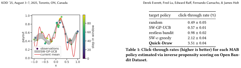
- On simulated nonstationary fields the policy outperforms sliding-window GP-UCB, sliding epsilon-greedy, and restless bandits, and on the Open Bandit Dataset it achieves a 65% relative improvement in click-through rate over the next-best baseline.
Reading between the lines
- The proof's requirement $\ell_x \le 1/\sqrt{T_{\max}-\rho^2}$ ties the spatial bandwidth to the horizon, so the constant $C$ in the regret bound grows with $T_{\max}$; the $\mathcal{O}^*(\sqrt{T})$ rate is therefore only proven up to a horizon-dependent constant, and for long runs the bound degrades to $O(T^{3/2})$ if $\ell_x$ is chosen as the theorem dictates.
- Because the estimator is a kernel interpolation estimator of the Nadaraya--Watson type, one could plug in other kernels (compact support, higher-order smoothness) and retain the same UCB structure, potentially extending the approach to reward classes beyond Lipschitz.
- The soft temporal decay in the variance is a form of forgetting; a testable extension is whether a sliding-window variant with a hard cutoff outperforms it when the reward changes abruptly rather than smoothly, since the Lipschitz-in-time assumption would then be violated.
Editorial analysis
A structured set of objections, weighed in public.
Referee Report
Summary. The paper introduces Quick-Draw, a UCB-type bandit policy for continuous arm spaces with many arms. The policy estimates the mean reward via a product of Gaussian likelihoods whose precision decays with spatial (and, in the non-stationary variant, temporal) distance, giving a kernel-interpolation mean and a closed-form variance. The authors claim an O*(sqrt T) cumulative regret bound for stationary Lipschitz reward functions (Theorems 4.1 and 4.2), and support the method with synthetic experiments on non-stationary random fields and an off-policy evaluation on the Open Bandit Dataset, emphasizing 100-10000x speedups over GP baselines.
Significance. The algorithmic idea is simple, computationally attractive (O(T) update with cached precisions), and the experiments address a practically relevant regime of many arms and non-stationarity. However, the paper's central theoretical contribution, the O*(sqrt T) regret guarantee, is not supported: the proof contains a reversed inequality, the bandwidth condition in Theorem 4.1 makes the constant horizon-dependent and destroys the claimed rate, and the claimed rate is in tension with the known Omega(T^{2/3}) lower bound for 1-D Lipschitz bandits. The empirical results are also presented without error bars, so the paper's headline contributions do not hold as written.
major comments (5)
- [Appendix B.2, proof of Theorem 4.2] The step 'Since sqrt(t) <= sqrt(T)' to conclude sum_t Sigma_t <= (1/sqrt(T)) sum_t C is reversed: because 1/sqrt(t) >= 1/sqrt(T), the sum is at least C sqrt(T), not at most. This invalidates the claimed upper bound of 8C^2 sqrt(T) ln^2(2T^2/delta) and is a load-bearing error in the central regret theorem.
- [Section 4, Theorem 4.1 and Theorem 4.2] The condition l_x <= 1/sqrt(Tmax - rho^2) forces l_x to shrink as Tmax grows. Since C = sqrt(rho^2 + 1/l_x^2), C grows like sqrt(Tmax). Substituting into the regret bound gives O(Tmax sqrt(T) log^2 T) at T = Tmax, i.e., O(T^{3/2}), not O*(sqrt T). The statement that 'Tmax can be arbitrarily large' therefore does not yield a uniform rate, and the abstract claim of O*(sqrt T) regret is unsupported.
- [Section 5, experiments] The experiments set l_x = l_t = 1 with Tmax = 1000 (e.g., Figures 3, 8, and 9), while Theorem 4.1 requires l_x <= 1/sqrt(1000 - rho^2) approximately 0.0316 for rho^2 = 1e-7. The theoretical guarantee therefore does not apply to the reported settings, so the empirical evaluation cannot be interpreted as a validation of the proven regret bound.
- [Abstract and Section 1] The claimed O*(sqrt T) rate for Lipschitz reward functions is in tension with the known minimax lower bound Omega(T^{2/3}) for 1-D Lipschitz bandits (see [15] in the paper). No additional assumption beyond Lipschitzness is identified that would justify this rate, so the abstract claim cannot be correct for the stated problem class unless an unstated condition is added.
- [Section 5 and Section 6] The empirical plots (Figures 4-9) report averages over 100 random payout functions but do not show standard errors or confidence bands, and the text claims 'statistically significant improvements' without reporting the relevant statistical tests. This makes it difficult to assess the robustness of the empirical comparisons.
minor comments (5)
- [Appendix B.1, proof of Lemma 4] The expression '4C1 sqrt((ln T+1)(ln(2T^2/delta) ln(2T^2/delta))' contains a malformed parenthesis and a duplicated logarithmic factor; please rewrite this line cleanly.
- [Section 5] The sentence 'the restless bandit policy significantly performs all other baselines' should read 'outperforms all other baselines'.
- [Throughout] The notation gamma_T is defined with a subscript T but used as gamma_{T+1} in several places; please make the indexing consistent.
- [Section 5, Figures 4-9] The captions for Figures 4-9 do not identify which curve corresponds to which policy; add a legend or clarify in the text.
- [Section 3, Eq. (1) and Eq. (3)] The parameter rho^2 is called the 'irreducible sampling error,' but it also appears in the non-stationary variance term; clarify whether rho^2 is intended to absorb time-discretization effects as well.
Circularity Check
No circularity: the regret derivation is standard UCB concentration machinery, and the identified concerns are proof-validity and parameter-dependence issues rather than circular reductions.
full rationale
The paper's derivation chain is self-contained with respect to the circularity patterns checked. The Quick-Draw index is defined by the Gaussian-interpolation variance model in Eqs. (1)-(3); the concentration inequality in Theorem 4.1 (Appendix B.1) is proved from the Lipschitz assumption, the variance model, and Freedman's martingale inequality (Lemma 5, citing an external reference [11]). The per-round regret bound in Lemma 1 is imported from standard external UCB literature ([26], [28]), not from the authors' own prior work, and it is not load-bearing in a self-referential way. The final regret bound in Theorem 4.2 is a direct summation of these per-round bounds. No fitted parameter is relabeled as a prediction, and no central claim rests on a self-citation chain. The theorem's condition l_x <= 1/sqrt(Tmax - rho^2) (Theorem 4.1) does make the constant C horizon-dependent, and the proof of Theorem 4.2 in Appendix B.2 contains a reversed summation inequality that undermines the stated O*(sqrt T) rate; however, these are correctness and parameterization weaknesses, not cases where the conclusion is assumed as an input. The paper also transparently acknowledges that its mean function is a Nadaraya-Watson kernel estimator, so there is no renaming of a known result presented as novel. Accordingly, no specific circular step can be quoted or exhibited.
Assumptions & free parameters
free parameters (4)
- rho^2 =
1e-7 in experiments
- l_x =
1 in experiments; theory requires l_x <= 1/sqrt(Tmax-rho^2)
- l_t =
1 in experiments
- gamma =
not stated for experiments; theory sets 2L + 4C_1 ln^2(2T^2/delta)
assumptions (5)
- domain assumption Mean payout mu(x,t) is Lipschitz in space and time with constant L
- domain assumption Rewards are zero-mean symmetric noise around mu with |epsilon| <= 1
- ad hoc to paper The conditional likelihood P(mu(x)|D_s) is Normal with variance rho^2 + distance^2/l^2
- standard math Freedman's martingale concentration inequality
- domain assumption Metric space distances are normalized to D <= 1
Cite this review
Pith. "Pith review of Quick-Draw Bandits: Quickly Optimizing in Nonstationary Environments with Extremely Many Arms." pith.science (2026). https://pith.science/paper/A3W6DXSA
@misc{pith2026250524692,
  author       = {Pith},
  title        = {Pith review of: Quick-Draw Bandits: Quickly Optimizing in Nonstationary Environments with Extremely Many Arms},
  year         = {2026},
  howpublished = {\url{https://pith.science/paper/A3W6DXSA}},
  note         = {Machine review of arXiv:2505.24692}
}
abstract
Canonical algorithms for multi-armed bandits typically assume a stationary reward environment where the size of the action space (number of arms) is small. More recently developed methods typically relax only one of these assumptions: existing non-stationary bandit policies are designed for a small number of arms, while Lipschitz, linear, and Gaussian process bandit policies are designed to handle a large (or infinite) number of arms in stationary reward environments under constraints on the reward function. In this manuscript, we propose a novel policy to learn reward environments over a continuous space using Gaussian interpolation. We show that our method efficiently learns continuous Lipschitz reward functions with $\mathcal{O}^*(\sqrt{T})$ cumulative regret. Furthermore, our method naturally extends to non-stationary problems with a simple modification. We finally demonstrate that our method is computationally favorable (100-10000x faster) and experimentally outperforms sliding Gaussian process policies on datasets with non-stationarity and an extremely large number of arms.
Figures


Figures from the paper (7 more)




Reference graph
Works this paper leans on
-
[15]
Nearly tight bounds for the continuum-armed bandit problem
Kleinberg, R. Nearly tight bounds for the continuum-armed bandit problem. Advances in Neural Information Processing Systems 17 (2004)
work page 2004
-
[1]
Sample mean based index policies with o(log n) regret for the multi- armed bandit problem
Agrawal, R. Sample mean based index policies with o(log n) regret for the multi- armed bandit problem. Advances in applied probability 27 , 4 (1995), 1054–1078
work page 1995
-
[2]
Ambikasaran, S., Foreman-Mackey, D., Greengard, L., Hogg, D. W., and O’Neil, M. Fast direct methods for gaussian processes. IEEE transactions on pattern analysis and machine intelligence 38 , 2 (2015), 252–265
work page 2015
-
[3]
Finite-time analysis of the multi- armed bandit problem
Auer, P., Cesa-Bianchi, N., and Fischer, P. Finite-time analysis of the multi- armed bandit problem. Machine learning 47 (2002), 235–256
work page 2002
-
[4]
Improved rates for the stochastic continuum-armed bandit problem
Auer, P., Ortner, R., and Szepesvári, C. Improved rates for the stochastic continuum-armed bandit problem. In International Conference on Computational Learning Theory (2007), Springer, pp. 454–468
work page 2007
-
[5]
Advances in neural information processing systems 34 (2021), 3004–3015
Bogunovic, I., and Krause, A.Misspecified gaussian process bandit optimization. Advances in neural information processing systems 34 (2021), 3004–3015
work page 2021
-
[6]
Products and convolutions of gaussian probability density functions
Bromiley, P. Products and convolutions of gaussian probability density functions. Tina-Vision Memo 3, 4 (2003), 1
work page 2003
-
[7]
Online optimization in x-armed bandits
Bubeck, S., Stoltz, G., Szepesvári, C., and Munos, R. Online optimization in x-armed bandits. Advances in Neural Information Processing Systems 21 (2008)
work page 2008
Show all 35 references
-
[8]
Bubeck, S., Stoltz, G., and Yu, J. Y. Lipschitz bandits without the lipschitz constant. In Algorithmic Learning Theory: 22nd International Conference, ALT 2011, Espoo, Finland, October 5-7, 2011. Proceedings 22 (2011), Springer, pp. 144–158
2011
-
[9]
Weighted gaussian process bandits for non-stationary environments
Deng, Y., Zhou, X., Kim, B., Tewari, A., Gupta, A., and Shroff, N. Weighted gaussian process bandits for non-stationary environments. In International Conference on Artificial Intelligence and Statistics (2022), PMLR, pp. 6909–6932
2022
-
[10]
High-dimensional gaussian process bandits
Djolonga, J., Krause, A., and Cevher, V. High-dimensional gaussian process bandits. Advances in neural information processing systems 26 (2013)
2013
-
[11]
Freedman, D. A. On tail probabilities for martingales. the Annals of Probability (1975), 100–118
1975
-
[12]
On upper-confidence bound policies for non- stationary bandit problems
Garivier, A., and Moulines, E. On upper-confidence bound policies for non- stationary bandit problems. arXiv preprint arXiv:0805.3415 (2008)
2008 arXiv
-
[13]
G., and Thompson, D
Horvitz, D. G., and Thompson, D. J. A generalization of sampling without replacement from a finite universe. Journal of the American statistical Association 47, 260 (1952), 663–685
1952
-
[14]
Jia, S., Xie, Q., Kallus, N., and Frazier, P. I. Smooth non-stationary bandits. In International Conference on Machine Learning (2023), PMLR, pp. 14930–14944
2023
-
[16]
Multi-armed bandits in metric spaces
Kleinberg, R., Slivkins, A., and Upfal, E. Multi-armed bandits in metric spaces. In Proceedings of the fortieth annual ACM symposium on Theory of computing (2008), pp. 681–690
2008
-
[17]
Bandits and experts in metric spaces
Kleinberg, R., Slivkins, A., and Upfal, E. Bandits and experts in metric spaces. Journal of the ACM (JACM) 66 , 4 (2019), 1–77
2019
-
[18]
Discounted ucb
Kocsis, L., and Szepesvári, C. Discounted ucb. In 2nd PASCAL Challenges Workshop (2006), vol. 2, pp. 51–134
2006
-
[19]
Algorithms for multi-armed bandit problems
Kuleshov, V., and Precup, D. Algorithms for multi-armed bandit problems. arXiv preprint arXiv:1402.6028 (2014)
2014 arXiv
-
[20]
L., and Robbins, H
Lai, T. L., and Robbins, H. Asymptotically efficient adaptive allocation rules. Advances in applied mathematics 6 , 1 (1985), 4–22
1985
-
[21]
Gstools v1
Müller, S., Schüler, L., Zech, A., and Hesse, F. Gstools v1. 3: a toolbox for geostatistical modelling in python. Geoscientific Model Development 15 , 7 (2022), 3161–3182
2022
-
[22]
A.On estimating regression.Theory of Probability & Its Applications 9, 1 (1964), 141–142
Nadaraya, E. A.On estimating regression.Theory of Probability & Its Applications 9, 1 (1964), 141–142
1964
-
[23]
Scikit-learn: Machine learning in python
Pedregosa, F., V aroqaux, G., Gramfort, A., Michel, V., Thirion, B., Grisel, O., Blondel, M., Prettenhofer, P., Weiss, R., Dubourg, V., et al. Scikit-learn: Machine learning in python. the Journal of machine Learning research 12 (2011), 2825–2830
2011
-
[24]
Weighted linear bandits for non- stationary environments
Russac, Y., Vernade, C., and Cappé, O. Weighted linear bandits for non- stationary environments. Advances in Neural Information Processing Systems 32 (2019)
2019
-
[25]
arXiv preprint arXiv:2008.07146 (2020)
Saito, Y., Aihara, S., Matsutani, M., and Narita, Y.Large-scale open dataset, pipeline, and benchmark for bandit algorithms. arXiv preprint arXiv:2008.07146 (2020)
2020 arXiv
-
[26]
Introduction to multi-armed bandits
Slivkins, A., et al. Introduction to multi-armed bandits. Foundations and Trends® in Machine Learning 12 , 1-2 (2019), 1–286
2019
-
[27]
Adapting to a changing environment: the brownian restless bandits
Slivkins, A., and Upfal, E. Adapting to a changing environment: the brownian restless bandits. In COLT (2008), pp. 343–354
2008
-
[28]
M., and Seeger, M
Srinivas, N., Krause, A., Kakade, S. M., and Seeger, M. Gaussian process optimization in the bandit setting: No regret and experimental design. arXiv preprint arXiv:0912.3995 (2009)
2009 arXiv
-
[29]
S., and Barto, A
Sutton, R. S., and Barto, A. G. Reinforcement learning: An introduction. Robotica 17, 2 (1999), 229–235
1999
-
[30]
Thompson, W. R. On the likelihood that one unknown probability exceeds another in view of the evidence of two samples. Biometrika 25, 3-4 (1933), 285– 294
1933
-
[31]
Thompson, W. R. On the theory of apportionment. American Journal of Mathe- matics 57, 2 (1935), 450–456
1935
-
[32]
Optimal order simple regret for gaussian process bandits
Vakili, S., Bouziani, N., Jalali, S., Bernacchia, A., and Shiu, D.-s. Optimal order simple regret for gaussian process bandits. Advances in Neural Information Processing Systems 34 (2021), 21202–21215
2021
-
[33]
Bandit convex optimization in non-stationary environments
Zhao, P., Wang, G., Zhang, L., and Zhou, Z.-H. Bandit convex optimization in non-stationary environments. Journal of Machine Learning Research 22 , 125 (2021), 1–45
2021
-
[34]
A simple approach for non- stationary linear bandits
Zhao, P., Zhang, L., Jiang, Y., and Zhou, Z.-H. A simple approach for non- stationary linear bandits. In International Conference on Artificial Intelligence and Statistics (2020), PMLR, pp. 746–755
2020
-
[35]
No-regret algorithms for time-varying bayesian optimization
Zhou, X., and Shroff, N. No-regret algorithms for time-varying bayesian optimization. In 2021 55th Annual Conference on Information Sciences and Systems (CISS) (2021), IEEE, pp. 1–6. A POLICY EXPLORATION/EXPLOITATION VIA HYPERPARAMETERS The behavior of the Quick-Draw policy is...
2021
Reviewed August 7, 2026 · model on record in the stance chip above.
Discussion (0). Sign in to comment.