REVIEW 3 major objections 5 minor 1 cited by
Sampled-data Systems: Stability, Contractivity and Single-iteration Suboptimal MPC
T0 review · 3 major / 5 minor · reviewed 2026-08-07 · deepseek-v4-flash
Pith's one-line read One optimization iteration per sample can keep MPC stable if the sampling period is small enough.
desk verdict Worth refereeing: the n=1 MPC stability result is real, the core proof is mostly solid, and the known gaps are fixable presentation issues plus a global-contractivity scope limit. read the letter →
The pith
A machine-rendered reading of the paper's core claim, the machinery that carries it, and where it could break.
The reading
What carries the argument
The load-bearing construct is the reduced model: the fictitious continuous-time system $\dot{x}=f(x,z^*(x))$ in which $z^*(x)=\lim_{n\to\infty}G^n(x,z)$ is the fixed point of the solver map, representing the ideal limit of infinitely fast sampling and infinitely many iterations. The argument then tracks the sampled-data dynamics through a $2\times2$ nonnegative matrix $A(n,T)$ (defined in Remark 8) whose entries are products of the contraction rate $\zeta$, the Lipschitz constants of $f$ and $G$, and the integral $h(T,\xi)=\int_0^T e^{\xi(T-s)}ds$; stability is reduced to showing this matrix is Schur stable, which is exactly what the threshold inequality $h(T,\xi)<(1-[\mathrm{Lip}_z(G)]^n)/(C_2(n)+C_1/\zeta)$ enforces. Solving this inequality for $T$ yields the explicit threshold $T(n)$ in (16), and the composite-norm machinery (weighted $\ell^2$ norms built from Perron eigenvectors) converts Schur stability of $A(n,T)$ into a discrete-time contraction bound, which Proposition 3.3 then lifts to a global exponential stability bound for all $t\ge0$.
What would settle it
Run a numerical continuation on the paper's first MPC example (double integrator with $A=[[0,1],[0,0]]$, $B=[0,1]^\top$, $\Delta=0.2$, horizon $H=5$, $R=1$, $Q=I$, $P$ from the DARE) with $n=1$: compute $T(1)$ explicitly from (16) and simulate the closed loop at $T=0.9\,T(1)$ and $T=1.1\,T(1)$ across a grid of initial conditions. Stability of all trajectories at $0.9\,T(1)$ and instability at $1.1\,T(1)$ supports the formula; conversely, any initial condition producing divergence at $T< T(1)$ under the stated assumptions would refute Theorem 3.6. A sharper falsification would search over the parameter space for any pair $(f,G)$ satisfying Assumptions 1-3 and contractivity of the reduced model for which the sampled loop is unstable for a sequence $T_k\to0$.
Extended reading notes
Core claim
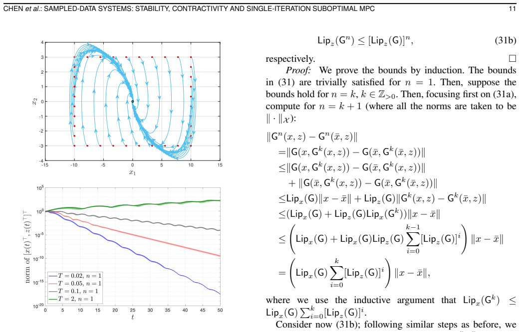
The paper's main theoretical result, Theorem 3.6, establishes that the sampled-data interconnection of a continuous-time system $\dot{x}=f(x,z)$ and a discrete-time map $z_k=G^n(x(kT),z_{k-1})$ is globally exponentially stable whenever the discrete map $z\mapsto G(x,z)$ is a contraction and the reduced model $\dot{x}=f(x,z^*(x))$ -- the limiting system obtained as $T\to0^+$ and $n\to+\infty$ -- is strongly infinitesimally contracting with rate $\zeta>0$. For each iteration count $n\ge1$, the paper produces a positive threshold $T(n)$, depending only on $n$ and on Lipschitz constants of $f$ and $G$, such that stability holds for all sampling periods $T<T(n)$; the threshold is explicitly computed in equation (16) and is shown to be increasing in $n$ and bounded above by a constant independent of $n$. Applied to model predictive control with a gradient-descent solver, this yields the claim that a single solver iteration per sample ($n=1$) preserves closed-loop stability whenever $T$ is sufficiently small, which the authors note is the first rigorous guarantee of this kind and is in contrast to earlier time-distributed MPC analyses that required more iterations. Under the stronger conditions that both the CT map and the DT map are contractive and satisfy the small-gain inequality $-\mathrm{osLip}_x(f)(1-\mathrm{Lip}_z(G))>\mathrm{Lip}_z(f)\mathrm{Lip}_x(G)$, Theorem 3.4 gives exponential stability and discrete-time contractivity for every $n$ and every $T>0$, with the small-gain condition shown in Theorem 3.5 to imply contractivity of the reduced model.
Load-bearing premise
The proof requires the reduced model to be globally uniformly contracting on the whole forward-invariant state set, meaning the ideal feedback law shrinks the distance between any two trajectories at a rate at least $\zeta$ everywhere; if this fails even locally, the paper's main theorem only gives a local stability result whose region of validity must be verified numerically.
Editorial extensions
If this is right
- For any MPC problem whose ideal closed-loop map is contractive, stability of the online implementation holds for every fixed iteration count $n$, including $n=1$, once the sampling period is below the computable threshold $T(n)$.
- Increasing the number of solver iterations per sample strictly enlarges the admissible sampling period, since $T(n)$ is increasing in $n$; the payoff of extra computation is a less demanding real-time update rate.
- The small-gain condition of Theorem 3.4 guarantees stability with no constraint on $T$ or $n$ at all, at the price of requiring the open plant map $x\mapsto f(x,z)$ to be contractive uniformly in $z$.
- For linear time-invariant systems, Theorem 3.6 upgrades to discrete-time contractivity of the sampled loop, not merely exponential stability, whenever the reduced-model matrix $A+B(I-D)^{-1}C$ is Hurwitz and $D$ is Schur.
- The explicit threshold formula gives a quantitative engineering guideline: the maximum allowable sensing-and-computation delay is expressible directly from plant and solver Lipschitz data, without solving LMIs or simulating the nonlinear loop.
Reading between the lines
- The same threshold logic should carry over to other operator-splitting or proximal solvers whose iteration maps are contractions with known Lipschitz constants, such as ADMM loops, suggesting a general recipe: certify contractivity of the ideal feedback law, then bound the sampling period by $T(n)$ computed from the solver's contraction factor.
- The monotonicity of $T(n)$ in $n$ suggests a natural online adaptation law: if the available compute time per sample grows, the controller can either increase $n$ or increase $T$ while preserving stability; the explicit trade-off curve $T(n)$ makes this a one-dimensional scheduling problem.
- Because contractivity of the reduced model is typically only local for constrained MPC (as the paper's own $\gamma=100$ experiment shows), the practically useful statement will be the local version, Corollary 3.7, whose forward-invariance condition currently must be checked numerically; a Lyapunov-function or barrier certificate that certifies the required set invariance would turn the result into
- The paper's Example 3.1, showing that any fixed $T$ can be destabilizing for an unstable open-loop plant, implies that the threshold $T(n)$ necessarily depends on the plant's unstable dynamics; controllers that aggressively stabilize may require extremely small $T$ at $n=1$, so the practical value of the single-iteration guarantee hinges on whether the required $T(1)$ is achievable in hardware.
Editorial analysis
A structured set of objections, weighed in public.
Referee Report
Summary. The paper studies the sampled-data interconnection of a continuous-time plant ẋ=f(x,z) with a discrete-time map z_k = G^n(x(kT), z_{k-1}), where z is held constant between sampling instants. It introduces a reduced model ẋ=f(x,z*(x)) obtained as T→0^+ and n→∞, and proves three groups of results: (i) Theorem 3.6, which states that if the DT map is contractive and the reduced model is strongly infinitesimally contracting, then for every n there is a threshold T(n) such that the CT-DT interconnection is globally exponentially stable for all T<T(n), with an explicit formula for T(n); (ii) Theorem 3.4, a small-gain condition implying discrete-time contractivity and exponential stability for all T and n; and (iii) an application to suboptimal MPC, arguing that a single iteration of the solver per sampling period suffices for stability when T is small. The proofs are based on contraction theory, Lipschitz/one-sided Lipschitz constants, and Schur-stability analysis of a 2×2 nonnegative matrix.
Significance. If the main results hold, the paper gives a useful quantitative bridge between continuous-time contraction of a reduced model and robust stability of a sampled-data implementation with finite solver iterations. The explicit T(n) expression, its monotonicity in n, and the comparison between small-gain and reduced-model conditions are valuable design insights. The proof of Theorem 3.6 is detailed: the Schur-condition algebra is carried through carefully, and the identities C1C2=C12C21 and C1[Lip_z(G)]^n = Lip_z(f)C21 used in the proof check out. The MPC application addresses a timely question, and the numerical experiments illustrate the qualitative behavior. However, as detailed below, the explicit threshold formula has a domain issue, the sign convention in Proposition 3.3 makes a displayed decay estimate incorrect as written, and the MPC claim for constrained/soft-constrained cases is broader than what the stated theorems actually support.
major comments (3)
- [III-C, Proposition 3.3 and Eq. (11)] The statement defines c := T^{-1} ln b. Since b∈(0,1), this c is negative, and the displayed bound ∥y(t)∥ ≤ r e^{-ct} ∥y(0)∥ is then an increasing exponential, not a decay. The proof repeats the same sign by writing c := ln b^{1/T} < 0 and then using e^{-c(kT+τ)}. The intended rate is certainly c := -T^{-1} ln b > 0, which is exactly what Remark 6 uses when it writes a := -T^{-1} ln ρ(A(n,T)). This is a load-bearing sign error in a stated implication, though it is locally fixable.
- [III-D, Theorem 3.6, Eq. (16)] The formula for T(n) is not always defined or positive. When ξ<0, the equation h(T,ξ) = R with R := (1-[Lip_z(G)]^n)/(C2(n)+C1/ζ) has a positive solution only if ξ R + 1 > 0; if R ≥ 1/(-ξ), then the argument of the logarithm in (16) is non-positive and the formula is meaningless. In the latter case the stability condition h(T,ξ)<R actually holds for every T>0, because h(T,ξ) is bounded above by 1/(-ξ). The theorem should either state T(n) as the infimum of T satisfying the condition, allowing T(n)=+∞ in this case, or add a hypothesis ensuring ξ R + 1 > 0. As written, the claims after (16) that T(n)>0 for all n and that T(n) is bounded by (17) are not valid on the full stated domain.
- [IV-B2, Corollary 3.7 and Figs. 6-7] The constrained MPC claim goes beyond what the stated results establish. Theorem 3.6 assumes global exponential contraction of the reduced model: osLip_x(f(x,z*(x))) ≤ -ζ on the forward-invariant set X. The paper's own Fig. 6 (right panel, γ=100) shows that this condition fails for large constraint penalties, and the text explicitly states that contractivity is not global. Corollary 3.7 does not actually relax the contraction assumption to a local one: it still assumes osLip(f(x,z*(x))) ≤ -ζ and only localizes the initial conditions together with forward invariance of X0×Z0 in X×Z. In the γ=10 experiment, the paper verifies forward invariance only numerically for one (n,T) pair and does not verify the global (or even X0-local) contraction hypothesis that Corollary 3.7 requires. Consequently, the advertised conclusion that “single-iteration suboptimal MPC is stabilizing for sufficiently small T” is rigorously established only for globally contractive reduced models, e.g., the unconstrained LQ example in Section IV-B1, not for the constrained/soft-constrained setting presented as validation in Section IV-B2. The authors should either state a genuinely local version of Theorem 3.6 with osLip condition on X0 and forward invariance of X0, or restrict the MPC claim accordingly.
minor comments (5)
- [II-A, definition of osLip_w(G)] In the displayed definition of osLip_w(G), the denominator uses “∥v1-v2∥²” but v1 and v2 are not defined; it should be ∥w1-w2∥².
- [V-A, Lemma 5.4] The statement uses the norm ∥·∥_U for the input difference, but no norm on an input space U has been introduced; this should be ∥·∥_Z (or a norm on the input space should be defined).
- [III-D, Theorem 3.6] The constant C1 depends on Lip_x(f), but Lip_x(f) is not defined in Assumptions 1-3; the authors should explicitly define it as the minimal uniform-in-z Lipschitz constant of x↦f(x,z).
- [III-E, Proposition 3.8] The proof of Proposition 3.8 is omitted with only a sketch; given that the paper otherwise provides complete proofs, a brief derivation or a precise reference to the LTI Schur-stability argument would improve completeness.
- [Throughout] There are several typos, including “Lipchitz” for “Lipschitz” and “assets” for “asserts”; these should be corrected in a revision.
Circularity Check
No load-bearing circularity: Theorem 3.6 and the single-iteration MPC conclusion are derived from independent contractivity assumptions; the only flagged items are minor, non-load-bearing self-citations to Bullo's contraction monograph.
full rationale
The central claim, Theorem 3.6, is not circular. Its assumption is contractivity of the reduced model, osLip_x(f(x,z*(x))) <= -zeta, together with contraction of the DT map G. The proof in Section V-E bounds the x-error using the reduced-model flow (equation (37)-(38)) and bounds the z-error using the contraction of G^n (equation (40)), then combines these into the matrix A(n,T) and imposes Schur stability via Lemma 5.3. No equation used as an assumption is also the conclusion by construction; the result is a genuine small-T preservation theorem. The single-iteration MPC claim is simply the n=1 specialization of the theorem, and it is conditional on the RM being contractive. In the first MPC experiment (Section IV-B1), this contractivity is verified by computing mu_{2,P}(A_cl) = -0.4407, not fitted to the stability outcome. There is no fitted parameter renamed as a prediction. The second MPC experiment (Section IV-B2, Figure 6) shows that for large penalty gamma the RM is not globally contractive, so the paper explicitly falls back to the local Corollary 3.7. That corollary requires forward invariance of X0 x Z0, which the paper checks only numerically by phase portraits for one (n,T) pair rather than by a formal certificate. This is a stated scope limitation, not a circular step. The manuscript relies on Bullo's contraction monograph [4] and on [28] (which includes two of the present authors) for standard lemmas on weak pairings, log-norms, and weighted norms. These cited tools are parameter-free, have stated assumptions that do not include the theorem being proved, and are used as auxiliary estimates rather than as the source of the stability conclusion. Accordingly, the self-citations are minor and not load-bearing, and the derivation chain is otherwise self-contained.
Assumptions & free parameters
assumptions (5)
- domain assumption Assumptions 1 and 2: f and G are Lipschitz with bounded interconnection gains Lip_z(f), Lip_x(G).
- domain assumption Assumption 3: Lip_z(G) < 1, i.e., the DT iteration map is a contraction in z.
- domain assumption Reduced model contractivity: osLip_x(f(x,z*(x))) ≤ -ζ < 0 on the forward-invariant set X.
- domain assumption Forward invariance of X × Z for the interconnected system (1).
- standard math Standard contraction theory background from Bullo [4]: log-norms, weak pairings, Lemma 2.8, Lemma 2.22, Corollary 3.17.
Cite this review
Pith. "Pith review of Sampled-data Systems: Stability, Contractivity and Single-iteration Suboptimal MPC." pith.science (2026). https://pith.science/paper/A7J4HSAX
@misc{pith2026250518336,
  author       = {Pith},
  title        = {Pith review of: Sampled-data Systems: Stability, Contractivity and Single-iteration Suboptimal MPC},
  year         = {2026},
  howpublished = {\url{https://pith.science/paper/A7J4HSAX}},
  note         = {Machine review of arXiv:2505.18336}
}
abstract
This paper analyzes the stability of interconnected continuous-time (CT) and discrete-time (DT) systems coupled through sampling and zero-order hold mechanisms. The DT system updates its output at regular intervals $T>0$ by applying an $n$-fold composition of a given map. This setup is motivated by online and sampled-data implementations of optimization-based controllers - particularly model predictive control (MPC) - where the DT system models $n$ iterations of an algorithm approximating the solution of an optimization problem. We introduce the concept of a reduced model, defined as the limiting behavior of the sampled-data system as $T \to 0^+$ and $n \to +\infty$. Our main theoretical contribution establishes that when the reduced model is contractive, there exists a threshold duration $T(n)$ for each iteration count $n$ such that the CT-DT interconnection achieves exponential stability for all sampling periods $T < T(n)$. Finally, under the stronger condition that both the CT and DT systems are contractive, we show exponential stability of their interconnection using a small-gain argument. Our theoretical results provide new insights into suboptimal MPC stability, showing that convergence guarantees hold even when using a single iteration of the optimization algorithm - a practically significant finding for real-time control applications.
Figures


Figures from the paper (4 more)


Forward citations
Cited by 1 Pith paper
-
Suboptimal and Reduced-Order MPC via Timescale Separation
Framework for suboptimal reduced-order nonlinear MPC using timescale separation to guarantee recursive feasibility and exponential stability at sufficiently fast sampling rates.
Reference graph
Works this paper leans on
-
[1]
Singular perturbation method for reducing the model order in optimal control design,
P. Kokotovic and P. Sannuti, “Singular perturbation method for reducing the model order in optimal control design,”IEEE Trans. on Automatic Control, vol. 13, no. 4, pp. 377–384, 1968
work page 1968
-
[2]
Singular perturba- tions and order reduction in control theory—an overview,
P. V . Kokotovic, R. E. O’Malley Jr, and P. Sannuti, “Singular perturba- tions and order reduction in control theory—an overview,”Automatica, vol. 12, no. 2, pp. 123–132, 1976
work page 1976
-
[3]
On contraction analysis for non-linear systems,
W. Lohmiller and J.-J. E. Slotine, “On contraction analysis for non-linear systems,”Automatica, vol. 34, no. 6, pp. 683–696, 1998
1998
-
[4]
Bullo,Contraction Theory for Dynamical Systems, 1.2 ed
F. Bullo,Contraction Theory for Dynamical Systems, 1.2 ed. Kindle Direct Publishing, 2024. [Online]. Available: https://fbullo.github.io/ctds
work page 2024
-
[5]
Rawlings, D
J. Rawlings, D. Mayne, and M. Diehl,Model Predictive Control: Theory, Computation, and Design. Nob Hill Publishing, 2017
2017
-
[6]
From linear to nonlinear MPC: Bridging the gap via the real-time iteration,
S. Gros, M. Zanon, R. Quirynen, A. Bemporad, and M. Diehl, “From linear to nonlinear MPC: Bridging the gap via the real-time iteration,” International Journal of Control, vol. 93, no. 1, pp. 62–80, 2020
2020
-
[7]
Model predictive control: Theory and practice,
M. Morari, C. E. Garcia, and D. M. Prett, “Model predictive control: Theory and practice,”IFAC Proceedings Volumes, vol. 21, no. 4, pp. 1–12, 1988
work page 1988
-
[8]
Control barrier functions: Theory and applications,
A. D. Ames, S. Coogan, M. Egerstedt, G. Notomista, K. Sreenath, and P. Tabuada, “Control barrier functions: Theory and applications,” inEuropean Control Conference, 2019, pp. 3420–3431
2019
Show all 42 references
-
[9]
W. Xiao, C. G. Cassandras, and C. Belta,Safe Autonomy with Control Barrier Functions: Theory and Applications. Springer, 2023
2023
-
[10]
Control-Lyapunov and control-barrier func- tions based quadratic program for spatio-temporal specifications,
K. Garg and D. Panagou, “Control-Lyapunov and control-barrier func- tions based quadratic program for spatio-temporal specifications,” in IEEE Conference on Decision and Control, 2019, pp. 1422–1429
2019
-
[11]
Freeman and P
R. Freeman and P. V . Kokotovic,Robust Nonlinear Control Design: State-Space and Lyapunov Techniques. Springer, 2008. 16
2008
-
[12]
Online optimization as a feedback controller: Stability and tracking,
M. Colombino, E. Dall’Anese, and A. Bernstein, “Online optimization as a feedback controller: Stability and tracking,”IEEE Trans. on Control of Network Systems, vol. 7, no. 1, pp. 422–432, 2019
2019
-
[13]
Timescale sepa- ration in autonomous optimization,
A. Hauswirth, S. Bolognani, G. Hug, and F. D ¨orfler, “Timescale sepa- ration in autonomous optimization,”IEEE Trans. on Automatic Control, vol. 66, no. 2, pp. 611–624, 2020
2020
-
[14]
A real-time iteration scheme for nonlinear optimization in optimal feedback control,
M. Diehl, H. G. Bock, and J. P. Schl ¨oder, “A real-time iteration scheme for nonlinear optimization in optimal feedback control,”SIAM Journal on Control and Optimization, vol. 43, no. 5, pp. 1714–1736, 2005
2005
-
[15]
Distributed model predictive control with suboptimality and stability guarantees,
P. Giselsson and A. Rantzer, “Distributed model predictive control with suboptimality and stability guarantees,” inIEEE Conference on Decision and Control, 2010, pp. 7272–7277
2010
-
[16]
Real-time suboptimal model predictive control using a combination of explicit mpc and online optimization,
M. N. Zeilinger, C. N. Jones, and M. Morari, “Real-time suboptimal model predictive control using a combination of explicit mpc and online optimization,”IEEE Trans. on Automatic Control, vol. 56, no. 7, pp. 1524–1534, 2011
2011
-
[17]
Instant distributed MPC with reference governor,
M. Figura, L. Su, M. Inoue, and V . Gupta, “Instant distributed MPC with reference governor,”International Journal of Control, vol. 97, no. 4, pp. 662–672, 2024
2024
-
[18]
Instant MPC for linear systems and dissipativity-based stability analysis,
K. Yoshida, M. Inoue, and T. Hatanaka, “Instant MPC for linear systems and dissipativity-based stability analysis,”IEEE Control Systems Letters, vol. 3, no. 4, pp. 811–816, 2019
2019
-
[19]
Time- distributed optimization for real-time model predictive control: Stability, robustness, and constraint satisfaction,
D. Liao-McPherson, M. M. Nicotra, and I. Kolmanovsky, “Time- distributed optimization for real-time model predictive control: Stability, robustness, and constraint satisfaction,”Automatica, vol. 117, p. 108973, 2020
2020
-
[20]
An analysis of closed-loop stability for linear model predictive control based on time-distributed optimization,
D. Liao-McPherson, T. Skibik, J. Leung, I. Kolmanovsky, and M. M. Nicotra, “An analysis of closed-loop stability for linear model predictive control based on time-distributed optimization,”IEEE Trans. on Auto- matic Control, vol. 67, no. 5, pp. 2618–2625, 2021
2021
-
[21]
Suboptimal MPC with a com- putation governor: Stability, recursive feasibility, and applications to ADMM,
S. van Leeuwen and I. Kolmanovsky, “Suboptimal MPC with a com- putation governor: Stability, recursive feasibility, and applications to ADMM,”arXiv preprint arXiv:2411.07919, 2024
2024 arXiv
-
[22]
Sampled-data primal- dual gradient dynamics in model predictive control,
R. Moriyasu, S. Kawaguchi, and K. Kashima, “Sampled-data primal- dual gradient dynamics in model predictive control,”Automatica, vol. 183, p. 112621, 2026
2026
-
[23]
On the finite- time behavior of suboptimal linear model predictive control,
A. Karapetyan, E. C. Balta, A. Iannelli, and J. Lygeros, “On the finite- time behavior of suboptimal linear model predictive control,” inIEEE Conference on Decision and Control, 2023, pp. 5053–5058
2023
-
[24]
Closed-loop finite-time analysis of suboptimal online control,
——, “Closed-loop finite-time analysis of suboptimal online control,” IEEE Trans. on Automatic Control, 2025
2025
-
[25]
Sta- bility certificates for receding horizon games,
S. Hall, D. Liao-McPherson, G. Belgioioso, and F. D ¨orfler, “Sta- bility certificates for receding horizon games,”arXiv preprint arXiv:2404.12165, 2024
2024 arXiv
-
[26]
A unified framework for input- to-state stability in systems with two time scales,
A. R. Teel, L. Moreau, and D. Nesic, “A unified framework for input- to-state stability in systems with two time scales,”IEEE Trans. on Automatic Control, vol. 48, no. 9, pp. 1526–1544, 2003
2003
-
[27]
A contraction theory approach to singularly perturbed systems,
D. Del Vecchio and J.-J. E. Slotine, “A contraction theory approach to singularly perturbed systems,”IEEE Trans. on Automatic Control, vol. 58, no. 3, pp. 752–757, 2012
2012
-
[28]
Online feedback optimiza- tion and singular perturbation via contraction theory,
L. Cothren, F. Bullo, and E. Dall’Anese, “Online feedback optimiza- tion and singular perturbation via contraction theory,”arXiv preprint arXiv:2310.07966, 2023
2023 arXiv
-
[29]
Contraction analysis of nonlinear DAE systems,
H. D. Nguyen, T. L. Vu, J.-J. Slotine, and K. Turitsyn, “Contraction analysis of nonlinear DAE systems,”IEEE Transactions on Automatic Control, vol. 66, no. 1, pp. 429–436, 2020
2020
-
[30]
A contraction approach to the hierarchical analysis and design of networked systems,
G. Russo, M. Di Bernardo, and E. D. Sontag, “A contraction approach to the hierarchical analysis and design of networked systems,”IEEE Trans. on Automatic Control, vol. 58, no. 5, pp. 1328–1331, 2012
2012
-
[31]
Sensitivity conditioning: Beyond singular perturbation for control design on multiple time scales,
M. Picallo, S. Bolognani, and F. D ¨orfler, “Sensitivity conditioning: Beyond singular perturbation for control design on multiple time scales,” IEEE Trans. on Automatic Control, vol. 68, no. 4, pp. 2309–2324, 2022
2022
-
[32]
Stability and stabilization of networked control systems,
W. Heemels and N. Van De Wouw, “Stability and stabilization of networked control systems,” inNetworked Control Systems. Springer, 2010, pp. 203–253
2010
-
[33]
A framework for stabilization of nonlinear sampled-data systems based on their approximate discrete-time models,
D. Nesic and A. R. Teel, “A framework for stabilization of nonlinear sampled-data systems based on their approximate discrete-time models,” IEEE Trans. on automatic control, vol. 49, no. 7, pp. 1103–1122, 2004
2004
-
[34]
On the robust stability and stabilization of sampled-data systems: A hybrid system approach,
P. Naghshtabrizi, J. P. Hespanha, and A. R. Teel, “On the robust stability and stabilization of sampled-data systems: A hybrid system approach,” inIEEE Conference on Decision and Control, 2006, pp. 4873–4878
2006
-
[35]
Robust stability and performance analysis of sampled-data systems,
N. Sivashankar and P. P. Khargonekar, “Robust stability and performance analysis of sampled-data systems,”IEEE Trans. on Automatic Control, vol. 38, no. 1, pp. 58–69, 1993
1993
-
[36]
A discrete-time approach to stability analysis of systems with aperiodic sample-and-hold devices,
H. Fujioka, “A discrete-time approach to stability analysis of systems with aperiodic sample-and-hold devices,”IEEE Trans. on Automatic Control, vol. 54, no. 10, pp. 2440–2445, 2009
2009
-
[37]
Sampled-data control of Lur’e systems,
G. W. Gabriel and J. C. Geromel, “Sampled-data control of Lur’e systems,”Nonlinear Analysis: Hybrid Systems, vol. 40, p. 100994, 2021
2021
-
[38]
Stability anal- ysis of sampled-data systems with sector-bounded input nonlinearity,
A. S. Fagundes, J. M. G. da Silva Jr, and S. Tarbouriech, “Stability anal- ysis of sampled-data systems with sector-bounded input nonlinearity,” IFAC-PapersOnLine, vol. 56, no. 2, pp. 9812–9817, 2023
2023
-
[39]
H. K. Khalil,Nonlinear Systems. Prentice Hall, 2002
2002
-
[40]
Sur les op ´erations dans les ensembles abstraits et leur application aux ´equations int´egrales,
S. Banach, “Sur les op ´erations dans les ensembles abstraits et leur application aux ´equations int´egrales,”Fundamenta Mathematicae, vol. 3, no. 1, pp. 133–181, 1922
1922
-
[41]
Un teorema generale sull’esistenza di elementi uniti in una transformazione funzionale,
R. Caccioppoli, “Un teorema generale sull’esistenza di elementi uniti in una transformazione funzionale,”Rendiconti dell’Accademia Nazionale dei Lincei, vol. 11, pp. 794–799, 1930
1930
-
[42]
Modularity, evolution, and the binding problem: a view from stability theory,
J.-J. Slotine and W. Lohmiller, “Modularity, evolution, and the binding problem: a view from stability theory,”Neural networks, vol. 14, no. 2, pp. 137–145, 2001
2001
Reviewed August 7, 2026 · model on record in the stance chip above.
Discussion (0). Continue with ORCID to comment.