REVIEW 3 major objections 5 minor 32 references
Deep learning of point processes for modeling high-frequency data
T0 review · 3 major / 5 minor · reviewed 2026-08-16 · deepseek-v4-flash
Pith's one-line read This paper proves an oracle inequality showing that deep neural networks can predict point-process intensities at a near-minimax rate, and demonstrates that a marked ratio model beats a joint model on simulated and real limit order book…
desk verdict This paper is a solid extension of Schmidt-Hieber's deep learning theory to point process intensities under alpha-mixing, with a genuine two-step marked-ratio estimator, but the stated rate does not cover the long-memory covariate used in the real-data application. read the letter →
The pith
A machine-rendered reading of the paper's core claim, the machinery that carries it, and where it could break.
The reading
What carries the argument
The central object is the contrast function $\Psi_T(a,b)=-\int_0^T a(X_t)\cdot dN_t+\int_0^T b(X_t)\,dt$, whose population expectation is used to define the risk. A compatibility condition makes the discrepancy $U(x)=-\lambda^*(x)\cdot(a(x)-a^*(x))+b(x)-b^*(x)$ nonnegative and comparable to the squared error, so minimizing $\Psi_T$ is a legitimate proxy for prediction. The proof then proceeds through a large-deviation lemma for additive functionals of geometrically $\alpha$-mixing processes, which controls the empirical-process terms, and a $\delta$-net covering-number bound for the neural network class, which controls complexity. For the applications, the marked ratio model factorizes the intensity into a baseline, a type component, and mark probabilities; the paper contrasts a one-step estimator of the joint marked ratio with a two-step estimator that fits each factor separately.
What would settle it
Simulate the marked ratio model with an intensity of the same functional form but drive one covariate by a long-memory process such as fractional Ornstein-Uhlenbeck, fit the two-step network, and measure the empirical risk at growing horizons: if the risk decays materially slower than the predicted rate $\phi_T$ up to logarithmic factors, the geometric-mixing assumption is essential to the bound. Alternatively, estimate the $\alpha$-mixing coefficients of the real book-imbalance and trade-sign series and check whether they decay exponentially.
Extended reading notes
Core claim
The paper establishes that the expected prediction error of the empirical contrast estimator for a point process with periodically stationary, geometrically $\alpha$-mixing covariates obeys $$R_T \le 2\Delta_T + 2\inf_{(a,b)\in\mathcal{F}_T} $h^{{-1}}$\mathbb{E}[\Psi_h(a,b)-\Psi_h(a^*,b^*)] + C_0(1+$F^{2}$)($T^{{-1}}$(\log T)^2\log N_T + \delta),$$ where $\Delta_T$ is the optimization error, the infimum is the approximation error, and $N_T$ is the covering number of the model class. In the deep-learning case with sparse ReLU networks whose size grows with $T$, this yields $R_T \le C\phi_T L(\log T)^4$, with $\phi_T = \max_i T^{-2\beta_i^*/(2\beta_i^*+t_i)}$ the effective smoothness rate, under the condition that the optimization error stays at the same order. The same framework covers Cox-type models, marked point processes, and multivariate point processes as special cases. The paper's empirical claim is that when the true intensity has the marked ratio factorization $\lambda_{i,k_i}(t)=\lambda_0(t)\lambda_i(X_t)p^i_{k_i}(Y_t)$, fitting the factors separately gives lower risk than estimating the joint intensity, and this holds both in simulation and on high-frequency limit order book data.
Load-bearing premise
The load-bearing assumption is that the covariate process $X$ is geometrically $\alpha$-mixing, meaning its dependence at lag $k$ decays like $e^{-\gamma k}$; if real covariates such as the sign of the last trade have long memory, the stated rate bound does not follow.
Editorial extensions
If this is right
- Any intensity model estimated by minimizing $\Psi_T$ inherits the same three-term oracle bound, so the theory covers non-network families as well as deep networks.
- With sparse ReLU networks of growing size, the risk converges at rate $\phi_T L(\log T)^4$, which is minimax-optimal up to logarithmic factors; the extra $(\log T)^4$ over the i.i.d. case is the price of the mixing dependence.
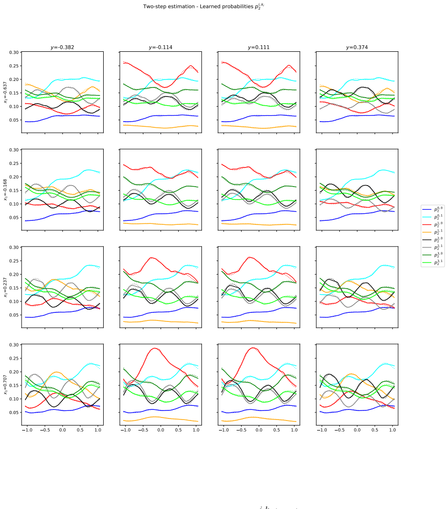
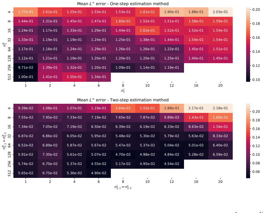
- The two-step marked ratio estimator gives lower $L^2$, $L^\infty$, and empirical-risk errors than the one-step estimator across simulation horizons, and the advantage persists across many network widths and depths.
- On real limit order book data, the fitted deep marked ratio model reproduces known microstructure regularities: imbalance and spread shape the probability of buy versus sell and price-changing versus non-price-changing market orders.
- Because the model is nonparametric, the same network architecture can in principle capture nonlinear covariate effects that fixed parametric families such as exponential intensities cannot express.
Reading between the lines
- The paper stops short of testing the rate theorem on data; a direct check would be to simulate a long-memory covariate process with a known intensity and compare the empirical risk decay to the predicted $\phi_T$ rate.
- The factorized-marked-ratio principle suggests a general design rule for point-process deep learning: encode known multiplicativity in the architecture. One can test this beyond the ratio model, for instance in state-dependent Hawkes or queue-reactive models where a similar factorization is plausible.
- The theorem assumes geometric $\alpha$-mixing, but the paper's real-data covariate, the sign of the last trade, is described as long-memory. Extending the large-deviation lemma to slowly mixing or long-range dependent inputs would be the natural next step and would determine whether the stated rate applies to the motivating application.
Signed reviews
Editorial analysis
A structured set of objections, weighed in public.
Referee Report
Summary. The paper studies nonparametric estimation of the intensity of a multivariate counting process when the intensity is a function of a covariate process, and uses deep ReLU networks as the estimating class. The loss is a general contrast function Ψ_T(a,b), and the risk is the expected contrast evaluated at the true intensity. Under a compatibility condition (2.1) relating the contrast to an L2-type discrepancy, a metric condition (2.3), and a geometric α-mixing assumption on the covariate process, Theorem 2.4 gives an oracle inequality: R_T is bounded by the optimization error Δ_T, the approximation error inf_{FT} h^{-1}E[Ψ_h(a,b)-Ψ_h(a*,b*)], and a complexity term of order (1+F^2)(T^{-1}(log T)^2 log N_T + δ). Theorem 3.1 combines this with Schmidt-Hieber-type network approximation and covering-number estimates to obtain R_T ≤ C φ_T L (log T)^4. The paper then introduces a marked ratio model, studies it in simulations with Ornstein-Uhlenbeck covariates, and applies it to Euronext limit order book data using imbalance, spread, and the sign of the last trade as covariates.
Significance. If the rates hold, this is a useful extension of the i.i.d. deep-learning regression theory of Schmidt-Hieber to point-process intensities under dependence. The oracle inequality cleanly separates optimization error, approximation error, and network complexity, and the proof of Theorem 2.4 is detailed and structurally coherent, using external large-deviation and covariance inequalities in a plausible way. The compatibility condition is checked for the principal examples, and the marked-ratio decomposition is practically motivated. The simulation design is transparent and the real-data application is realistic. The main caveats are the mismatch between the geometric-mixing premise and the long-memory last-trade-sign covariate used in the real-data analysis, and the fact that the multi-output networks used in the simulations are not explicitly covered by the p_L=1 statement in Section 3.
major comments (3)
- [Section 4.2 and Theorem 2.4] The geometric α-mixing condition on the covariate process X is load-bearing for Theorem 2.4, entering through Lemmas 5.1, 5.3 and 5.4. In the real-data application, Section 4.2 includes X^1_t as the sign of the last trade and states that trade signs have long memory. A stationary binary process with hyperbolically decaying autocorrelation cannot be geometrically α-mixing, so the stated rate bound cannot be invoked for the LOB analysis. The authors should either verify the mixing condition for the actual covariates used (or at least discuss its plausibility empirically), or explicitly state that the real-data section is heuristic and outside the scope of the rate theorem.
- [Section 2, mixing coefficient definition] The mixing condition is printed as α_X^h(k) ≤ γ^{-1} e^{-γ h} for all k ∈ Z_+, with the right-hand side independent of k. As written, this does not express decay of the α-mixing coefficients in k. The covariance bound (5.23) and the subsequent large-deviation estimates require geometric decay in k; the condition should presumably read γ^{-1} e^{-γ k} (or an equivalent). This is a load-bearing assumption in the theorem statement and should be corrected.
- [Section 3 versus Sections 4.1.2-4.1.3] Section 3 states that p_L=1 for the applications in the article, but the one-step and two-step estimation methods in Section 4 use networks with output dimensions 7 and 3, respectively. The softmax normalization couples the output coordinates, and the theorem as stated with p_L=1 does not explicitly cover this multi-output architecture. Please either state a multi-output version of Theorem 3.1 with the corresponding approximation and covering-number bounds, or explain that the simulation estimates each scalar ratio function separately with p_L=1 networks. This does not affect Theorem 2.4, which is architecture-independent, but it affects the claim that Theorem 3.1 directly justifies the numerical experiments.
minor comments (5)
- [Section 4.1.5 and Figure 6] The simulation comparison reports means over 20 samples without standard errors or confidence bands. Since the two-step method is claimed to be clearly superior, adding error bars or a formal comparison at each horizon would strengthen the empirical claim.
- [Section 2 and Section 5] The notation for the horizon is confusing: T ∈ T is sometimes used as a continuous time length and sometimes as an integer in conditions such as T ≥ 3 ∨ log N_T. The proof uses T = T/h; please introduce a separate symbol for the number of blocks or clarify the convention in the theorem statements.
- [Section 5.1, Eq. (5.1)] There is a typographical error in the definition of R_T^e: the displayed expression has a mismatched expectation bracket. Please correct it.
- [Section 4.1.1] The baseline intensity λ_0(t)=1+cos(2πt) has period 1, but the period h of the periodic stationarity is not specified in the simulation. Please state the value of h used in the experiments and its relation to the theoretical block length.
- [Remark 3.2(ii)] The minimax-optimality claim is justified through the independent-input submodel. Since the theorem's class contains independent covariates, the lower-bound argument is valid, but the wording could be made more precise by saying the lower bound is obtained for the submodel with periodically independent covariates.
Circularity Check
No circularity: the oracle inequality is derived from explicit contrast and mixing assumptions using independent external results.
full rationale
The central bound (2.4) is not an input restated as an output. It is proved in Section 5 by decomposing R_T into an empirical error R_T - R^e_T and the expected contrast gap, then bounding the two fluctuation terms Phi_T^(5.3) and Phi_T^(5.4) through Lemmas 5.1-5.4. Lemma 5.1 uses a Bernstein-type large-deviation inequality of Merlevede et al. [13] and Rio's covariance inequality [21] under the explicitly stated geometric alpha-mixing condition on X; Lemmas 5.3 and 5.4 estimate the second moments of L_T and M_T from those bounds. The approximation and covering-number estimates (3.3)-(3.4) are taken from Schmidt-Hieber [22], an independent published result, and from a compatibility condition (2.2) that is verified rather than assumed to contain the conclusion. No fitted constant enters Theorem 2.4 or Theorem 3.1 except through the covering number and the optimization-error hypothesis Delta_T <= C_0 phi_T L (log T)^4, which is stated as a sufficient condition, not derived as a prediction. The self-citations Muni Toke and Yoshida [16,17,18] motivate the ratio/marked-ratio contrast examples and the LOB application, but they are not used as premises in the proof of the oracle inequality or the convergence rate. The empirical rate comparison in Section 4.1.5 is descriptive, and its reference slopes are explicitly labeled 'for visual guidance,' so it is not a disguised reproducibility of the theorem. The possible incompatibility of geometric alpha-mixing with the long-memory trade-sign covariate in Section 4.2 is an applicability gap between assumptions and a real-data example, not a circular reduction: the theorem remains a conditional statement for processes satisfying the mixing assumption. Hence there is no circular step and the derivation is self-contained with respect to its stated assumptions.
Assumptions & free parameters
free parameters (4)
- h (block length) =
chosen by user; constants depend on it
- δ (covering radius) =
free parameter in the oracle inequality
- network size (L, widths p_l, sparsity s, bound F) =
functions of T satisfying (3.2), e.g., s ≍ T φ_T log T
- ξ =
arbitrary positive
assumptions (7)
- domain assumption Intensity representation λ_t = λ(X_t) with bounded λ and no common jumps among components.
- domain assumption Periodic stationarity of (X_j) and geometric α-mixing of X: α_X^h(k) ≤ γ^{-1} e^{-γ k} for some γ > 0.
- domain assumption Compatibility condition (2.1): U(x) is nonnegative and comparable to squared L2 distance between (a,b) and (a*,b*).
- ad hoc to paper Metric condition (2.3): d lower bounds the sup-norm distance times a constant.
- domain assumption The target is in the Hölder composition class G(q,d,t,β,K) and satisfies the Schmidt-Hieber network conditions (3.2).
- domain assumption Optimization error bound ∆T ≤ C0 φ_T L (log T)^4.
- domain assumption Membership (a*,b*) ∈ A and F_T ⊂ A with sup-norm bound F.
Cite this review
Pith. "Pith review of Deep learning of point processes for modeling high-frequency data." pith.science (2026). https://pith.science/paper/AIQL4N3L
@misc{pith2026250415944,
  author       = {Pith},
  title        = {Pith review of: Deep learning of point processes for modeling high-frequency data},
  year         = {2026},
  howpublished = {\url{https://pith.science/paper/AIQL4N3L}},
  note         = {Machine review of arXiv:2504.15944}
}
read the original abstract
We investigate applications of deep neural networks to a point process having an intensity with mixing covariates processes as input. Our generic model includes Cox-type models and marked point processes as well as multivariate point processes. An oracle inequality and a rate of convergence are derived for the prediction error. A simulation study shows that the marked point process can be superior to the simple multivariate model in prediction. We apply the marked ratio model to real limit order book data
Figures


Figures from the paper (7 more)




Reference graph
Works this paper leans on
-
[1]
application to high frequency financial data
Bacry, E., Dayri, K., Muzy, J.F.: Non-parametric kernel estimation for symmetric Hawkes processes. application to high frequency financial data. The European Physical Journal B 85, 1–12 (2012)
work page 2012
-
[2]
Quantitative Finance 13(1), 65–77 (2013)
Bacry, E., Delattre, S., Hoffmann, M., Muzy, J.F.: Modelling microstructure noise with mutually exciting point processes. Quantitative Finance 13(1), 65–77 (2013)
work page 2013
-
[3]
Journal of Econometrics 141(2), 876–912 (2007)
Bowsher, C.G.: Modelling security market events in continuous time: Intensity based, multivariate point process models. Journal of Econometrics 141(2), 876–912 (2007)
work page 2007
-
[4]
Acta Numerica 30, 327 – 444 (2021)
DeVore, R., Hanin, B., Petrova, G.: Neural network approximation. Acta Numerica 30, 327 – 444 (2021). DOI 10.1017/s0962492921000052. URL http://dx.doi.org/10.1017/ S0962492921000052
-
[5]
Statistical Science 36(2) (2021)
Fan, J., Ma, C., Zhong, Y.: A selective overview of deep learning. Statistical Science 36(2) (2021). DOI 10.1214/20-sts783. URL http://dx.doi.org/10.1214/20-STS783
-
[6]
Econometrica 89(1), 181 – 213 (2021)
Farrell, M.H., Liang, T., Misra, S.: Deep neural networks for estimation and inference. Econometrica 89(1), 181 – 213 (2021). DOI 10.3982/ecta16901. URL http://dx.doi. org/10.3982/ECTA16901
-
[7]
Imaizumi, M.: Sup-norm convergence of deep neural network estimator for nonparametric regression by adversarial training (2023). DOI 10.48550/ARXIV.2307.04042. URL https: //arxiv.org/abs/2307.04042
-
[8]
Kim, J., Nakamaki, T., Suzuki, T.: Transformers are minimax optimal nonparametric in-context learners (2024). DOI 10.48550/ARXIV.2408.12186. URL https://arxiv.org/ abs/2408.12186
Show all 32 references
-
[9]
Bernoulli 31(1) (2025)
Kurisu, D., Fukami, R., Koike, Y.: Adaptive deep learning for nonlinear time series models. Bernoulli 31(1) (2025). DOI 10.3150/24-bej1726. URL http://dx.doi.org/10.3150/ 24-BEJ1726
2025 doi
-
[10]
Journal of Financial Markets 10(1), 1–25 (2007)
Large, J.: Measuring the resiliency of an electronic limit order book. Journal of Financial Markets 10(1), 1–25 (2007)
2007
-
[11]
Quantitative Finance 18(2), 249–264 (2018)
Lu, X., Abergel, F.: High-dimensional Hawkes processes for limit order books: modelling, empirical analysis and numerical calibration. Quantitative Finance 18(2), 249–264 (2018)
2018
-
[12]
Quantitative Finance 22(11), 1989–2003 (2022) 33
Maglaras, C., Moallemi, C.C., Wang, M.: A deep learning approach to estimating fill probabilities in a limit order book. Quantitative Finance 22(11), 1989–2003 (2022) 33
2022
-
[13]
In: High dimensional probability V: the Luminy volume, vol
Merlevede, F., Peligrad, M., Rio, E.: Bernstein inequality and moderate deviations under strong mixing conditions. In: High dimensional probability V: the Luminy volume, vol. 5, pp. 273–293. Institute of Mathematical Statistics (2009)
2009
-
[14]
Quantitative Finance 22(3), 563–583 (2022)
Morariu-Patrichi, M., Pakkanen, M.S.: State-dependent Hawkes processes and their appli- cation to limit order book modelling. Quantitative Finance 22(3), 563–583 (2022)
2022
-
[15]
Economics discussion paper (2011-32) (2011)
Muni Toke, I., Pomponio, F.: Modelling trades-through in a limited order book using Hawkes processes. Economics discussion paper (2011-32) (2011)
2011
-
[16]
Quantitative Finance 17(5), 683–701 (2017)
Muni Toke, I., Yoshida, N.: Modelling intensities of order flows in a limit order book. Quantitative Finance 17(5), 683–701 (2017)
2017
-
[17]
Quantitative Finance pp
Muni Toke, I., Yoshida, N.: Analyzing order flows in limit order books with ratios of Cox-type intensities. Quantitative Finance pp. 1–18 (2019)
2019
-
[18]
Japanese Journal of Statistics and Data Science 5(1), 1–39 (2022)
Muni Toke, I., Yoshida, N.: Marked point processes and intensity ratios for limit order book modeling. Japanese Journal of Statistics and Data Science 5(1), 1–39 (2022)
2022
- [19]
-
[20]
Quantitative Finance 17(7), 999–1020 (2017)
Rambaldi, M., Bacry, E., Lillo, F.: The role of volume in order book dynamics: a multi- variate Hawkes process analysis. Quantitative Finance 17(7), 999–1020 (2017)
2017
-
[21]
Springer (2017)
Rio, E.: Asymptotic Theory of Weakly Dependent Random Processes. Springer (2017)
2017
-
[22]
The Annals of Statistics 48(4), 1875 – 1897 (2020)
Schmidt-Hieber, J.: Nonparametric regression using deep neural networks with ReLU activation function. The Annals of Statistics 48(4), 1875 – 1897 (2020). DOI 10.1214/ 19-AOS1875. URL https://doi.org/10.1214/19-AOS1875
2020 doi
-
[23]
Market Microstructure and Liquidity (2023)
Sfendourakis, E., Muni Toke, I.: Lob modeling using Hawkes processes with a state- dependent factor. Market Microstructure and Liquidity (2023)
2023
-
[24]
SIAM (2009)
Shorack, G.R., Wellner, J.A.: Empirical processes with applications to statistics. SIAM (2009)
2009
-
[25]
Quantitative Finance 19(4), 549–570 (2019)
Sirignano, J.A.: Deep learning for limit order books. Quantitative Finance 19(4), 549–570 (2019)
2019
- [26]
-
[27]
Advances in Neural Information Processing Systems 34, 3609–3621 (2021) 34
Suzuki, T., Nitanda, A.: Deep learning is adaptive to intrinsic dimensionality of model smoothness in anisotropic besov space. Advances in Neural Information Processing Systems 34, 3609–3621 (2021) 34
2021
-
[28]
In: 2017 IEEE 19th conference on business informatics (CBI), vol
Tsantekidis, A., Passalis, N., Tefas, A., Kanniainen, J., Gabbouj, M., Iosifidis, A.: Fore- casting stock prices from the limit order book using convolutional neural networks. In: 2017 IEEE 19th conference on business informatics (CBI), vol. 1, pp. 7–12. IEEE (2017)
2017
-
[29]
Market microstructure and liquidity (2022)
Wu, P., Rambaldi, M., Muzy, J.F., Bacry, E.: Queue-reactive Hawkes models for the order flow. Market microstructure and liquidity (2022)
2022
-
[30]
Yoshida, N.: Polynomial type large deviation inequalities and quasi-likelihood analysis for stochastic differential equations. Ann. Inst. Statist. Math. 63(3), 431–479 (2011). DOI 10.1007/s10463-009-0263-z. URL http://dx.doi.org/10.1007/s10463-009-0263-z
2011 doi
-
[31]
Annals of the Institute of Statistical Mathematics pp
Yoshida, N.: Simplified quasi-likelihood analysis for a locally asymptotically quadratic random field. Annals of the Institute of Statistical Mathematics pp. 1–24 (2024)
2024
-
[32]
Zhang, Z., Zohren, S., Roberts, S.: Deeplob: Deep convolutional neural networks for limit order books. IEEE Transactions on Signal Processing 67(11), 3001–3012 (2019) Appendix 35 1 2 4 6 8 10 12 16 20 nL 1 48163264128256512 nN 1 6.87e-02 6.71e-02 6.96e-02 7.46e-02 7.46e-02 8.2...
2019
Reviewed August 16, 2026 · model on record in the stance chip above.
Discussion (0). Continue with ORCID to comment.