Analytical approximations of dispersion laws and ultra-complex conductivity diagrams

A.Ya. Maltsev

REVIEW 3 major objections 4 minor 50 references

Analytical approximations of dispersion laws and ultra-complex conductivity diagrams

T0 review · 3 major / 4 minor · reviewed 2026-08-02 · deepseek-v4-flash

Challenge this review Re-run · record.json Download PDF Read on arXiv ↗ Review JSON

Pith's one-line read For simple and body-centered cubic tight-binding metals, the Fermi-energy window that generates ultra-complex conductivity diagrams is narrow: about 1.5% of the conduction band for the simple cubic lattice near δ=0.5, and at most about 1% o

desk verdict Plausible and clearly worked out, but the narrow-width headline rests on an unproven reduction from global extrema to two boundary points, so the numbers are lower bounds until that gap is closed. read the letter →

arxiv 2606.30004 v3 pith:AWCJ26IT submitted 2026-06-29 cond-mat.mtrl-sci

A.Ya. Maltsev This is my paper · ORCID

classification cond-mat.mtrl-sci

keywords tight-bindingapproximationultra-complexconductivitydiagramsopenelectrontrajectoriesFermisurfacetopologystrongmagneticfieldssimplecubiclatticebody-centeredstabilityzones

verification ladder T0 review T1 audit T2 compute T3 formal

The pith

A machine-rendered reading of the paper's core claim, the machinery that carries it, and where it could break.

The reading

This paper asks why the 'ultra-complex' conductivity diagrams predicted for electron motion in strong magnetic fields have not been observed in experiments. Its answer is quantitative: for the simple and body-centered cubic lattices in the tight-binding approximation, the Fermi-energy interval [εB1, εB2] that produces such diagrams is very narrow. Including next-nearest-neighbor hopping, the paper estimates the width as about 1.5% of the conduction-band width for the simple cubic lattice near δ=0.5, and at most about 1% of the total band width (and less than a tenth of the complex-diagram interval) for the body-centered cubic lattice. The paper's contribution is thus a concrete, parameter-dependent explanation of the rarity of ultra-complex diagrams and a specification of where, in energy, one would still try to find them.

What carries the argument

The calculation is carried by the boundary-energy function ε~0(n): the Fermi-energy value at which a stability-zone boundary is reached and one of the closed-trajectory cylinders separating carriers of open trajectories collapses to zero height. A stability zone is a set of magnetic-field directions n for which the Fermi surface supports stable open trajectories for a whole interval of Fermi energies. The paper evaluates ε~0 only at two symmetric points P and Q on the boundary of the largest stability zone W1, translates the zero-height-cylinder condition into plane-tangency conditions on the Fermi surface, solves the resulting algebraic systems as functions of the next-nearest-neighbor hopp

What would settle it

For the two dispersions in the paper, compute the functions ε~1(n) and ε~2(n) numerically on a dense grid of magnetic-field directions at representative values (e.g., δ=0.5 for the simple cubic lattice and δ=0.6 for the body-centered cubic lattice), find the global minimum of ε~2 and the global maximum of ε~1 over the sphere, and compare them with the paper's ε~0(P), ε~0(Q) curves. If the global extrema occur at other boundary points, the true interval is wider than the estimated 1–1.5% and the low-probability conclusion would need revision.

Watch

Extended reading notes

Core claim

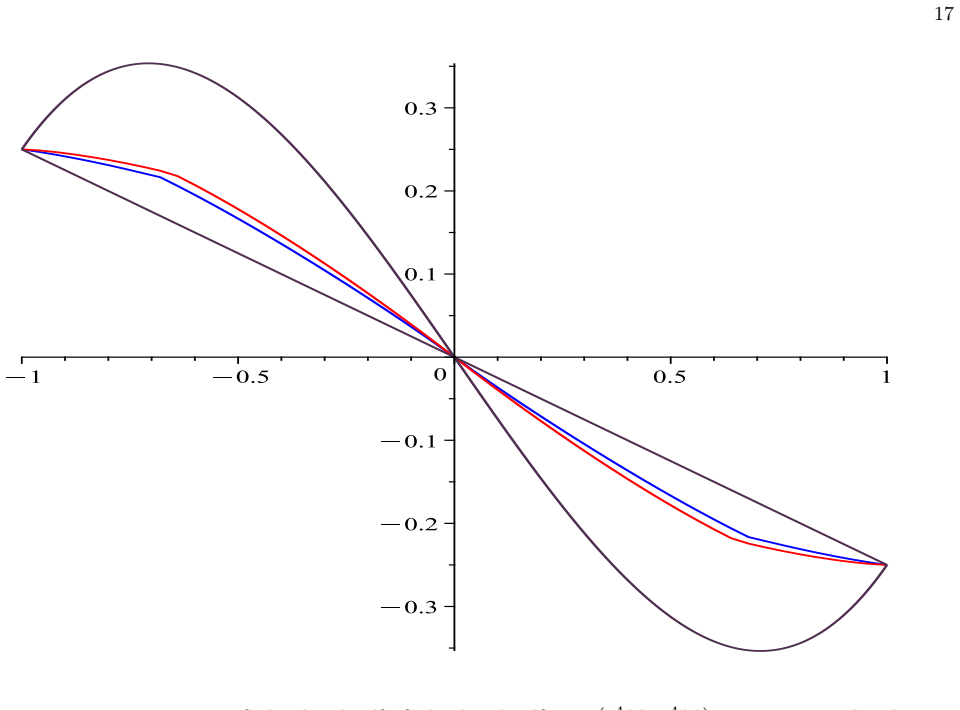
The paper establishes that higher-order corrections in the tight-binding expansion make the interval [εB1, εB2] non-degenerate but small. For the simple cubic lattice with dispersion εδ(p)=cos x+cos y+cos z + 2δ(cos x cos y + cos x cos z + cos y cos z), it gives [εB1, εB2] ≃ [ε~0(P), ε~0(Q)], with ε~0(P) < ε~0(Q) for 0<δ<0.5 and width on the order of 1.5% of the conduction-band width near δ=0.5. For the body-centered cubic lattice with dispersion εδ(p)=cos x cos y cos z + (δ/4)(cos 2x + cos 2y + cos 2z), the corresponding interval [ε~0(Q), ε~0(P)] lies inside the extended-Fermi-surface interval (εA1, εA2)=(-3δ/4+δ^3/2, -δ/4) for δ>0, and its width is at most 0.1 of that interval and at most

Load-bearing premise

The width and probability conclusion rests on the assumption that the two symmetric boundary points P and Q of the largest stability zone are where the boundary energy ε~0 attains its global minimum and maximum, so the interval between them equals [εB1, εB2] instead of merely being a subset of it.

Editorial extensions

If this is right

If the estimates are correct, the absence of experimental observations of ultra-complex diagrams is expected: the Fermi energy must fall within a band of roughly 1–1.5% of the band width.
For the body-centered cubic lattice, type B diagrams occur inside the extended-surface interval (εA1, εA2) but occupy less than a tenth of it, so only finely positioned Fermi levels produce them.
For the simple cubic lattice the window widens as δ approaches ±0.5, making materials with stronger next-nearest-neighbor hopping the most plausible candidates.
The sign symmetry δ→−δ, εF→−εF means the same narrow-window conclusion holds for negative hopping amplitudes with the Fermi-energy axis reversed.
The computed intervals give concrete energy targets: a conductor whose Fermi level can be moved through this narrow window should exhibit the anomalous magnetotransport associated with type B diagrams.

Reading between the lines

Editorial extensions of the paper, not claims the author makes directly.

The paper leaves open whether the two symmetric points P and Q actually realize the global extrema required by the exact definitions of εB1 and εB2; a numerical global search over the sphere could confirm that the estimated width is the true width rather than only a lower bound.
If real materials have next-nearest-neighbor hopping much smaller than δ≈0.5, the inferred width would shrink roughly proportionally, making ultra-complex diagrams even less likely; conversely, strain or pressure that changes effective hopping amplitudes could widen the window far enough to be observable.
The same boundary-energy method should transfer to other high-symmetry lattices, such as face-centered cubic or lattices with longer-range hoppings, whenever the leading-order dispersion has a degeneracy that collapses [εB1, εB2] to a point.

Share X Bluesky LinkedIn Reddit HN

Signed reviews

No signed human review yet.

Editorial analysis

A structured set of objections, weighed in public.

Desk editor's note, referee report, and a circularity audit.

Desk Editor's Note

read the letter

The thing to know: this paper gives a concrete way to estimate the width of the type-B (ultra-complex) conductivity interval for simple and body-centered cubic tight-binding dispersions with next-nearest-neighbor hopping. It extends the author's earlier work, where the interval collapsed to a point in leading order, and produces finite widths: about 1.5% of the band for SC near delta=0.5, and under 1% for BCC. The tangency systems (III.3)-(III.6) are explicit, internally consistent, and solved cleanly; the figures are informative. This is a useful technical step within the Novikov-Dynnikov magnetotransport program.

The soft spot is the key reduction. The exact definitions (II.1) are global extrema over the whole sphere, but the calculation replaces them by extrema over stability-zone boundaries and then evaluates epsilon_0 only at two symmetric points P and Q. That is asserted, not proved or numerically tested. The paper itself notes the inclusion for BCC: [epsilon_0(Q), epsilon_0(P)] is a subset of [epsilon_B1, epsilon_B2]. So the computed interval is, at best, a lower bound on the true interval. The conclusion that the interval 'does not exceed' 1% or 0.1 of the A-interval width doesn't follow from the computation as presented. The true interval could be wider if other boundary directions realize lower epsilon_B1 or higher epsilon_B2. The same issue affects the SC case. This is not a fatal flaw—the method is sensible and the numbers plausible—but it is load-bearing for the probability claim, and it is addressable with a direct numerical check on the full S^2 extrema or a proof that the boundary extrema reduce to P and Q.

There are two smaller caveats: the roots of the tangency systems have no error estimates, and the 'probability' interpretation implicitly assumes the Fermi level is uniformly distributed over the band, which is not stated or defended. Neither is disqualifying.

The paper is aimed at specialists in topological Fermi-surface physics and galvanomagnetic transport. It deserves a serious referee, but the referee should send it back for justification of the P/Q shortcut before the width numbers are used. If that gets fixed—or if the bound is restated as a lower bound—this becomes a solid contribution.

Recommendation: engage, but condition the accept on the reduction being verified.

Referee Report

3 major / 4 minor

Summary. The manuscript estimates the energy interval [εB1, εB2] in which "ultra-complex" (type B) conductivity diagrams occur, for tight-binding dispersion laws of simple cubic (SC) and body-centered cubic (BCC) lattices with next-nearest-neighbor hopping amplitude δ. The author replaces the exact global-extrema definitions of εB1 and εB2 (Eq. II.1) by extrema of the function ε̃₀ on stability-zone boundaries (Eq. II.2) and then by values at two symmetric boundary points P and Q of the largest stability zone W1. For the SC lattice, tangency conditions lead to the curves in Fig. 14, and the paper reports a width of about 1.5% of the conduction band width near δ = 0.5. For the BCC lattice, systems (III.3)–(III.6) yield Fig. 23, with a reported width of at most 0.1 of (εA1, εA2) and at most 1% of the full band. The Conclusion states that the probability of observing such diagrams in a given substance is quite low.

Significance. If the central reduction from global extrema to the two symmetric points P and Q is valid, the paper gives concrete, parameter-dependent quantitative predictions for a quantity that is extremely difficult to compute directly. The approach is not circular: the width is calculated from the dispersion law rather than fitted to the target interval. The tangency systems are written out explicitly, which is a strength, and the work connects a topological classification to a practical tight-binding calculation. However, the main numerical claims currently rest on an unproved and partly self-admitted approximation, so the significance is conditional on closing that gap.

major comments (3)

[§II–III, Eqs. (II.1)–(II.2), Figs. 14, 23] The width estimates are obtained by replacing the exact definitions εB1 = min_{S²} ε̃₂(n), εB2 = max_{S²} ε̃₁(n) with extrema of ε̃₀ over stability-zone boundaries (II.2), and then evaluating ε̃₀ only at the symmetric points P and Q. This reduction is asserted without proof or numerical verification. For the BCC case the paper itself states the inclusion [ε̃₀(Q), ε̃₀(P)] ⊆ [εB1, εB2], so the computed interval is, by the author's own admission, only a lower bound on the true type-B interval. Nevertheless, the Conclusion and Figs. 14 and 23 are used to state upper bounds ('does not exceed 0.1', 'does not exceed 1%'). Unless the global extrema are verified—by direct sampling over ∂Wα or by a symmetry argument—the 1–1.5% widths are not established as the widths of [εB1, εB2], and the 'quite low probability' conclusion is unsupported.
[§IV, Abstract] The probability claim is not operationalized. The only model parameter is δ, and no probability distribution over δ (or over material families) is specified. The width of the interval [εB1, εB2] for a fixed δ does not by itself determine the probability of occurrence in a given substance; one needs a measure on the space of dispersion-law parameters. As written, 'the probability ... is quite low' is a qualitative statement about a narrow two-parameter family, not a probability estimate in any statistical sense.
[§III, systems (III.3)–(III.6)] The paper states that systems (III.3)–(III.6) are independently solved and that the solution corresponding to the larger value of µ/ν is selected, but it gives no numerical values, no accuracy checks, and no demonstration that the selected branch satisfies the tangency conditions globally rather than only locally. Given that Fig. 23 is the main quantitative output for the BCC case, the absence of any numerical verification or reproducibility data makes the central claim difficult to audit. A table of computed ε̃₀(P,δ) and ε̃₀(Q,δ) for representative δ values, together with a direct check of the global extrema, would be a minimal addition.

minor comments (4)

[§II, Fig. 14] The phrase 'of the order of 1.5% of the conduction band width' is not defined precisely: is the reference width [εmin, εmax] of the full dispersion (II.3), or some other measure? A numerical table for ε̃₀(P) and ε̃₀(Q) at selected δ would remove the ambiguity.
[§III, Eq. (III.1)] The formula for the interval (εA1, εA2) = (−3δ/4 + δ³/2, −δ/4) is stated without derivation. A short proof or a reference to where this calculation appears would be helpful.
[General] The notation P/Q is used in opposite order in the SC and BCC sections: the SC interval is written [ε̃₀(P), ε̃₀(Q)] while the BCC interval is [ε̃₀(Q), ε̃₀(P)]. The figure captions and the text should define the ordering explicitly to avoid confusion.
[§II, last paragraph] The manuscript restricts the SC treatment to |δ| < 0.5, but the Conclusion refers to 'the simple cubic lattice' without this caveat. The restriction should be carried through the abstract and conclusion.

Circularity Check

2 steps flagged · score 4.0 of 10

P/Q shortcut and subset-to-interval inference rest on same-author self-citation [44]; reported narrow widths are not established bounds on [εB1, εB2].

ansatz smuggled in via citation [Section II, Eq. (II.2) and the paragraph following it]
"Here we use the method proposed in [44] and suitable for many relations ǫ(p) that have a fairly rich symmetry. Namely, we first replace the expressions (II.1) with the expressions ǫ_B^1 = min_{∪∂Wα} ε~0(n), ǫ_B^2 = max_{∪∂Wα} ε~0(n) (II.2) ... which give the same values of ǫ_B^1 and ǫ_B^2 for the majority of 'physically realistic' relationships ǫ(p). Second, to evaluate the expressions (II.2), we use the values of ε~0(P) and ε~0(Q) at the 'symmetric' points P and Q of the boundary of the symmetric Zone W1"

The exact interval is defined in (II.1) by global extrema over all of S². The paper reduces this to extrema over stability-zone boundaries (II.2) and then to the single pair P,Q on the boundary of W1, citing only [44] (the author's own prior work) and an unproved 'majority' assertion. No proof or numerical test is given that P,Q realize the global extrema; the narrow 1–1.5% widths therefore follow from the self-cited ansatz rather than from the defining equations. If [44] contains the missing proof, it is not reproduced here, so the load-bearing step is not independently verified.
other [Section III, paragraph beginning 'Here we use the intervals...']
"Here we use the intervals [ε~0(Q, δ), ε~0(P, δ)] (Fig. 8) to estimate the intervals [ε_B^1(δ), ε_B^2(δ)]. As we have already said, in the general case we have the inclusion [ε~0(Q, δ), ε~0(P, δ)] ⊆ [ε_B^1(δ), ε_B^2(δ)], moreover, for large Zones Wα these intervals coincide in order of magnitude (and often coincide exactly)."

For BCC the paper explicitly admits the computed interval is only a subset of the target interval. A subset's width is a lower bound, not an upper bound, for [εB1, εB2]. Nevertheless the Conclusion treats the subset width as bounding the true interval ('does not exceed 0.1 ... does not exceed 1%'), relying on the unproved clause 'for large Zones these intervals coincide in order of magnitude.' This is the same self-cited ansatz; the upper-bound result is assumed rather than derived.

full rationale

The exact quantity under study, [εB1, εB2], is defined by global extrema of ε~1 and ε~2 over S² (II.1). The paper's numerical work instead solves tangency conditions for the dispersion laws (II.3) and (III.1) at the two symmetric points P and Q on the boundary of the largest stability zone W1. These computations are not fitted to data and have genuine independent content. However, the reduction from the global-extrema definition to the boundary points is justified only by citing the author's own prior work [44] and by the assertion that the replacement 'give[s] the same values ... for the majority of physically realistic relationships.' No proof, numerical check, or error bound is supplied. For the BCC case the paper itself states the inclusion [ε~0(Q,δ),ε~0(P,δ)] ⊆ [εB1,εB2], which makes the computed width a lower bound on the subset rather than an upper bound on the true interval. The subsequent conclusion that the true interval is at most 1% of the band therefore depends on the unproved 'coincide in order of magnitude' clause. These issues make the load-bearing link between the computation and the stated conclusion reliant on a self-citation and an ansatz, but the central dispersion-based calculations are not themselves circular. Hence a moderate score of 4 is appropriate.

Assumptions & free parameters 1 free parameters · 4 assumptions · 0 invented entities

The quantitative claim rests on a truncated tight-binding model, on prior classification theorems for generic dispersions, and on an unproved reduction of exact stability-zone extrema to values at two symmetric points. No external data or numerical benchmark is used, so the ledger is dominated by domain assumptions rather than fitted numbers; δ is the only scanned model parameter.

free parameters (1)

δ (relative next-nearest-neighbor hopping amplitude) = scanned in (-0.5, 0.5) for simple cubic; (-1, 1) for body-centered cubic
Not fitted to any material; it is the model parameter controlling higher-order tight-binding corrections. The central width estimates depend strongly on δ, with maxima near δ ≈ 0.5 (simple cubic) and δ ≈ 0.6 (body-centered cubic).

assumptions (4)

domain assumption Tight-binding dispersion can be truncated to nearest- and next-nearest-neighbor hopping terms (Eqs. II.3 and III.1).
Higher Fourier harmonics are neglected; the width values depend on this truncation, and no convergence test against additional harmonics is provided.
domain assumption For δ ≠ 0 the dispersion is generic, so the type-A/type-B classification and stability-zone formalism of [27,28] apply.
The paper relies on prior classification results for generic dispersion relations and asserts that the higher-order corrections restore genericity (§II after Eq. II.3; §III: 'becomes a generic relation').
ad hoc to paper The exact extrema in (II.1) can be replaced by extrema over stability-zone boundaries (II.2), and then by values at the symmetric points P and Q of the largest zone W1.
This is the key approximation; it is asserted without proof or numerical verification and is load-bearing for all quantitative width estimates.
domain assumption Electron dynamics on the Fermi surface is given by (I.1) and conductivity asymptotics by (I.2)–(I.5), with the standard classification of stable open trajectories.
Standard Lifshitz–Novikov solid-state background taken from cited literature; not re-derived in this paper.

how reviews work

0 comments

Cite this review

Pith. "Pith review of Analytical approximations of dispersion laws and ultra-complex conductivity diagrams." pith.science (2026). https://pith.science/paper/AWCJ26IT

@misc{pith2026260630004,
  author       = {Pith},
  title        = {Pith review of: Analytical approximations of dispersion laws and ultra-complex conductivity diagrams},
  year         = {2026},
  howpublished = {\url{https://pith.science/paper/AWCJ26IT}},
  note         = {Machine review of arXiv:2606.30004}
}

read the original abstract

We study the probability of the emergence of ultra-complex conductivity diagrams in conductors that satisfy the tight-binding approximation and have the simple or body-centered cubic lattice. The presence of ultra-complex conductivity diagrams allows us to observe a number of highly nontrivial effects in strong magnetic fields, however, the probability of their emergence in a given substance is quite low. In the case of the simple or body-centered cubic lattice, the leading tight-binding approximation does not allow us to estimate this probability due to the peculiarities of the spectra in this situation. To estimate this probability, we use higher-order corrections to the leading approximation, which yield more accurate analytical expressions for the electron spectra.

Figures

Figures reproduced from arXiv: 2606.30004 by the authors.

**Figure 2.** FIG. 2: (a,b) Simple Fermi surfaces of electron and hole type [PITH_FULL_IMAGE:figures/full_fig_p003_2.png] view at source ↗

**Figure 3.** FIG. 3: (a) Abstract Fermi surfaces of genus 0, 1, 2, 3, and 4. ( [PITH_FULL_IMAGE:figures/full_fig_p004_3.png] view at source ↗

Figures from the paper (20 more)

**Figure 4.** Figure 4: FIG. 4: The shape of a stable open trajectory of system (I.1) [PITH_FULL_IMAGE:figures/full_fig_p004_4.png]

**Figure 5.** Figure 5: FIG. 5: (a) Complex angular diagram of type [PITH_FULL_IMAGE:figures/full_fig_p005_5.png]

**Figure 6.** Figure 6: FIG. 6: Type B diagrams (schematically). The signs [PITH_FULL_IMAGE:figures/full_fig_p005_6.png]

**Figure 7.** Figure 7: FIG. 7: (a) Chaotic trajectory of the Dynnikov type in a plane [PITH_FULL_IMAGE:figures/full_fig_p006_7.png]

**Figure 8.** Figure 8: FIG. 8: (a) Zones [PITH_FULL_IMAGE:figures/full_fig_p007_8.png]

**Figure 9.** Figure 9: FIG. 9: (a) Complex Fermi surface divided by closed trajecto [PITH_FULL_IMAGE:figures/full_fig_p007_9.png]

**Figure 10.** Figure 10: FIG. 10: Principal and additional jumps between nodes of a [PITH_FULL_IMAGE:figures/full_fig_p008_10.png]

**Figure 11.** Figure 11: FIG. 11: The Fermi surfaces [PITH_FULL_IMAGE:figures/full_fig_p009_11.png]

**Figure 12.** Figure 12: FIG. 12: Simultaneous tangency of a pair of ovals defined by th [PITH_FULL_IMAGE:figures/full_fig_p009_12.png]

**Figure 13.** Figure 13: FIG. 13: The level lines [PITH_FULL_IMAGE:figures/full_fig_p010_13.png]

**Figure 14.** Figure 14: FIG. 14: The values [PITH_FULL_IMAGE:figures/full_fig_p011_14.png]

**Figure 15.** Figure 15: FIG. 15: Main and additional jumps in the body-centered [PITH_FULL_IMAGE:figures/full_fig_p011_15.png]

**Figure 16.** Figure 16: FIG. 16: The Fermi surfaces (III.2) for [PITH_FULL_IMAGE:figures/full_fig_p012_16.png]

**Figure 17.** Figure 17: FIG. 17: The Fermi surfaces [PITH_FULL_IMAGE:figures/full_fig_p013_17.png]

**Figure 18.** Figure 18: FIG. 18: The Fermi surfaces [PITH_FULL_IMAGE:figures/full_fig_p013_18.png]

**Figure 19.** Figure 19: FIG. 19: (a) Cylinders [PITH_FULL_IMAGE:figures/full_fig_p014_19.png]

**Figure 20.** Figure 20: FIG. 20: Topological diagram of the connection of carri [PITH_FULL_IMAGE:figures/full_fig_p014_20.png]

**Figure 21.** Figure 21: FIG. 21: (a) Section of the Fermi surface [PITH_FULL_IMAGE:figures/full_fig_p015_21.png]

**Figure 22.** Figure 22: FIG. 22: (a) Section of the Fermi surface [PITH_FULL_IMAGE:figures/full_fig_p016_22.png]

**Figure 23.** Figure 23: FIG. 23: Boundaries of the intervals [PITH_FULL_IMAGE:figures/full_fig_p017_23.png]

Review history (3 revisions) →

Discussion (0). Continue with ORCID to comment.

Reference graph

Works this paper leans on

50 extracted references · 3 linked inside Pith

[1]

Each stable open trajectory of (I.1) lies in a straight strip of ﬁnite width (in a plane orthogonal to B), passing through it (Fig. 4)
[2]

wandering every- where

The mean direction of stable open trajectories in p - space is given by the intersection of the plane orthogo- nal to B and some integer (generated by two reciprocal lattice vectors) plane Γ , which is unchanged under small rotations of B . The contribution of stable open trajectories to the ten- sor σkl(B) is also strongly anisotropic in the plane or- th...
[3]

− − δ 2 cos √ 2c + δ 4 cos 2ν(c − π/ √
[4]

= ˜ǫ0(Q, δ) , 1 2 ( cos √ 2a + 1 ) cos(νa + ζ) + + δ 2 cos √ 2a + δ 4 cos 2(νa + ζ) = ˜ǫ0(Q, δ) , 1 2 ( cos √ 2b + cos √ 2h ) cos(νb + ζ) + + δ 2 cos √ 2b · cos √ 2h + δ 4 cos 2(νb +ζ) = ˜ǫ0(Q, δ) , ν ( cos √ 2c − 1 ) sin ν(c−π/ √
[5]

+ + √ 2 sin √ 2c cos ν(c−π/ √
[6]

22: (a) Section of the Fermi surface ǫδ(p) = ˜ǫ0(Q) by the planes Π1,2(B) containing the cylinders C − 1 and C + 1 , C + 2 of zero height

− √ 2δ sin √ 2c = 0 , ν ( cos √ 2a + 1 ) sin(νa + ζ) + νδ sin 2(νa + ζ) + + √ 2 sin √ 2a cos(νa + ζ) + √ 2δ sin √ 2a = 0 , cos(νb + ζ) + δ cos √ 2b = 0 , ν ( cos √ 2b + cos √ 2h ) sin(νb + ζ) + νδ sin 2(νb + ζ) + + √ 2 sin √ 2b cos(νb+ζ) + √ 2δ sin √ 2b cos √ 2h = 0 (III.5) 16 (B)Π 2 (B)Π 1 (B)Π z u z u A B C A C B a b FIG. 22: (a) Section of the Fermi su...
[7]

Kittel, Quantum Theory of Solids, Wiley, New York (1963)

C. Kittel, Quantum Theory of Solids, Wiley, New York (1963)

1963
[8]

Ziman, Principles of the Theory of Solids, Cam- bridge University Press 1972

J.M. Ziman, Principles of the Theory of Solids, Cam- bridge University Press 1972

1972

Show all 50 references

[9]

Ashcroft y N

N.W. Ashcroft y N. D. Mermin, Solid State Physics, Saunders Collage Publishing, 1976

1976
[10]

Abrikosov., Fundamentals of the Theory of Metals., Elsevier Science & Technology, Oxford, United Kingdom, 1988

A.A. Abrikosov., Fundamentals of the Theory of Metals., Elsevier Science & Technology, Oxford, United Kingdom, 1988

1988
[11]

Lifshitz, M.Ya

I.M. Lifshitz, M.Ya. Azbel, M.I. Kaganov., The Theory of Galvanomagnetic Eﬀects in Metals., Sov. Phys. JETP 4:1, 41-53 (1957)

1957
[12]

Lifshitz, V.G

I.M. Lifshitz, V.G. Peschansky., Galvanomagnetic char - acteristics of metals with open Fermi surfaces., Sov. Phys. JETP 8:5, 875-883 (1959)

1959
[13]

Lifshitz, V.G

I.M. Lifshitz, V.G. Peschansky., Galvanomagnetic char - acteristics of metals with open Fermi surfaces. II., Sov. Phys. JETP 11:1, 131-141 (1960)

1960
[14]

Lifshitz, M.Ya

I.M. Lifshitz, M.Ya. Azbel, M.I. Kaganov., Electron The - ory of Metals. New York: Consultants Bureau, 1973

1973
[15]

Novikov., The Hamiltonian formalism and a many- valued analogue of Morse theory., Russian Math

S.P. Novikov., The Hamiltonian formalism and a many- valued analogue of Morse theory., Russian Math. Surveys 37 (5), 1-56 (1982)

1982
[16]

Zorich., A problem of Novikov on the semiclassi- 18 cal motion of an electron in a uniform almost rational magnetic ﬁeld., Russian Math

A.V. Zorich., A problem of Novikov on the semiclassi- 18 cal motion of an electron in a uniform almost rational magnetic ﬁeld., Russian Math. Surveys 39 (5), 287-288 (1984)

1984
[17]

Dynnikov., Proof of S.P

I.A. Dynnikov., Proof of S.P. Novikov’s conjecture for the case of small perturbations of rational magnetic ﬁelds., Russian Math. Surveys 47:3, 172-173 (1992)

1992
[18]

Tsarev, private communication, 1992-1993

S.P. Tsarev, private communication, 1992-1993

1992
[19]

Dynnikov., Proof of S.P

I.A. Dynnikov., Proof of S.P. Novikov’s conjecture on t he semiclassical motion of an electron., Math. Notes 53:5, 495-501 (1993)

1993
[20]

Geometric Study of Foliations

A.V. Zorich., Proc. “Geometric Study of Foliations”., (Tokyo, November 1993) / ed. T.Mizutani et al. Singa- pore: World Scientiﬁc, 479-498 (1994)

1993
[21]

Dynnikov., Surfaces in 3-torus: geometry of plane sections., Proc

I.A. Dynnikov., Surfaces in 3-torus: geometry of plane sections., Proc. of ECM2, BuDA, 1996

1996
[22]

Dynnikov., Semiclassical motion of the electron

I.A. Dynnikov., Semiclassical motion of the electron. A proof of the Novikov conjecture in general position and counterexamples., Solitons, geometry, and topology: on the crossroad, Amer. Math. Soc. Transl. Ser. 2, 179, Amer. Math. Soc., Providence, RI, 1997, 45-73

1997
[23]

Dynnikov., The geometry of stability zones in Novikov’s problem on the semiclassical motion of an elec- tron., Russian Math

I.A. Dynnikov., The geometry of stability zones in Novikov’s problem on the semiclassical motion of an elec- tron., Russian Math. Surveys 54:1, 21-59 (1999)

1999
[24]

Novikov, A.Y

S.P. Novikov, A.Y. Maltsev, Topological quantum char- acteristics observed in the investigation of the conduc- tivity in normal metals., JETP Letters 63 (10), 855-860 (1996)

1996
[25]

Maltsev, Anomalous behavior of the electrical co n- ductivity tensor in strong magnetic ﬁelds., Journal of Experimental and Theoretical Physics 85 (5), 934-942 (1997)

A.Ya. Maltsev, Anomalous behavior of the electrical co n- ductivity tensor in strong magnetic ﬁelds., Journal of Experimental and Theoretical Physics 85 (5), 934-942 (1997)

1997
[26]

Novikov, A.Y

S.P. Novikov, A.Y. Maltsev, Topological phenomena in normal metals, Physics-Uspekhi 41:3, 231 (1998)

1998
[27]

A. Ya. Maltsev and S. P. Novikov, Quasiperiodic func- tions and dynamical systems in quantum solid state physics, Bulletin of Braz. Math. Society , New Series 34, 171 (2003)

2003
[28]

A. Ya. Maltsev and S. P. Novikov, Dynamical Systems, Topology, and Conductivity in Normal Metals, J. Stat. Phys. 115, 31 (2004)

2004
[29]

De Leo., Topological eﬀects in the magnetoresistanc e of Au and Ag., Phys

R. De Leo., Topological eﬀects in the magnetoresistanc e of Au and Ag., Phys. Lett. A 332, 469–474 (2004)

2004
[30]

R. De Leo., First-principles generation of stereograp hic maps for high-ﬁeld magnetoresistance in normal metals: An application to Au and Ag., Physica B: Condensed Matter 362 (1–4) (2005), 62–75

2005
[31]

Maltsev, S.P

A.Ya. Maltsev, S.P. Novikov., The Theory of Closed 1-Forms, Levels of Quasiperiodic Functions and Trans- port Phenomena in Electron Systems., Proceedings of the Steklov Institute of Mathematics 302, 279-297 (2018)

2018
[32]

Roberto De Leo., A survey on quasiperiodic topology., Advanced Mathematical Methods in Biosciences & Ap- plications, Springer, Eds. F. Berezovskaya and B. Toni, (2018)., arXiv:1711.01716

2018 arXiv
[33]

A.Ya. Maltsev, The second boundaries of stability zone s and the angular diagrams of conductivity for metals hav- ing complicated Fermi surfaces, Journal of Experimental and Theoretical Physics 127 (6), 1087-1111 (2018)

2018
[34]

Maltsev, The Complexity Classes of Angular Di- agrams of the Metal Conductivity in Strong Magnetic Fields, Journal of Experimental and Theoretical Physics 129(1), 116-138 (2019)

A.Ya. Maltsev, The Complexity Classes of Angular Di- agrams of the Metal Conductivity in Strong Magnetic Fields, Journal of Experimental and Theoretical Physics 129(1), 116-138 (2019)

2019
[35]

Dynnikov, A.Ya

I.A. Dynnikov, A.Ya. Maltsev, S.P. Novikov, Geometry of quasi-periodic functions on the plane, Russian Math. Surveys 77 : 6, 1061–1085 (2022), arXiv:2306.11257

2022 arXiv
[36]

Pseudoperiodic Topology

Anton Zorich, How do the leaves of closed 1-form wind around a surface., “Pseudoperiodic Topology”, V.I.Arnold, M.Kontsevich, A.Zorich (eds.), Translations of the AMS, Ser. 2, vol. 197, AMS, Providence, RI, 1999, 135-178

1999
[37]

De Leo., Existence and measure of ergodic leaves in Novikov’s problem on the semiclassical motion of an elec- tron., Russian Math

R. De Leo., Existence and measure of ergodic leaves in Novikov’s problem on the semiclassical motion of an elec- tron., Russian Math. Surveys 55:1 (2000), 166-168

2000
[38]

ergodic di- rections

R. De Leo., Characterization of the set of “ergodic di- rections” in Novikov’s problem of quasi-electron orbits in normal metals., Russian Math. Surveys 58:5 (2003), 1042-1043

2003
[39]

De Leo., Topology of plane sections of periodic poly- hedra with an application to the Truncated Octahedron., Experimental Mathematics 15:1 (2006), 109-124

R. De Leo., Topology of plane sections of periodic poly- hedra with an application to the Truncated Octahedron., Experimental Mathematics 15:1 (2006), 109-124

2006
[40]

De Leo, I.A

R. De Leo, I.A. Dynnikov., An example of a fractal set of plane directions having chaotic intersections with a ﬁxed 3-periodic surface., Russian Math. Surveys 62:5 (2007), 990-992

2007
[41]

Dynnikov, Interval identiﬁcation systems and pla ne sections of 3-periodic surfaces, Proceedings of the Steklov Institute of Mathematics 263, 65-77 (2008)

I.A. Dynnikov, Interval identiﬁcation systems and pla ne sections of 3-periodic surfaces, Proceedings of the Steklov Institute of Mathematics 263, 65-77 (2008)

2008
[42]

De Leo, I.A

R. De Leo, I.A. Dynnikov., Geometry of plane sections of the inﬁnite regular skew polyhedron {4, 6 | 4}., Geom. Dedicata 138:1 (2009), 51-67

2009
[43]

Skripchenko., Symmetric interval identiﬁcation sy s- tems of order three., Discrete Contin

A. Skripchenko., Symmetric interval identiﬁcation sy s- tems of order three., Discrete Contin. Dyn. Sys. 32:2 (2012), 643-656

2012
[44]

Skripchenko., On connectedness of chaotic sections of some 3-periodic surfaces., Ann

A. Skripchenko., On connectedness of chaotic sections of some 3-periodic surfaces., Ann. Glob. Anal. Geom. 43 (2013), 253-271

2013
[45]

Dynnikov, A

I. Dynnikov, A. Skripchenko., On typical leaves of a mea - sured foliated 2-complex of thin type., Topology, Ge- ometry, Integrable Systems, and Mathematical Physics: Novikov’s Seminar 2012-2014, Advances in the Mathe- matical Sciences., Amer. Math. Soc. Transl. Ser. 2, 234, e...

2012 arXiv
[46]

Dynnikov, A

I. Dynnikov, A. Skripchenko., Symmetric band com- plexes of thin type and chaotic sections which are not actually chaotic., Trans. Moscow Math. Soc. , Vol. 76, no. 2, 2015, 287-308

2015
[47]

A vila, P

A. A vila, P. Hubert, A. Skripchenko., Diﬀusion for chaotic plane sections of 3-periodic surfaces., Inventiones mathematicae, October 2016, Volume 206, Issue 1, pp 109–146

2016
[48]

A vila, P

A. A vila, P. Hubert, A. Skripchenko., On the Hausdorﬀ dimension of the Rauzy gasket., Bulletin de la societe mathematique de France , 2016, 144 (3), pp. 539 - 568

2016
[49]

Ivan Dynnikov, Pascal Hubert, Alexandra Skripchenko, Dynamical Systems Around the Rauzy Gasket and Their Ergodic Properties, International Mathematics Research 19 Notices IMRN Volume 2023, Issue 8, April 2023, Pages 6461–6503

2023
[50]

Maltsev, On chaotic regimes of conductiv- ity behavior in the tight-binding approximation, arXiv:2510.17589

A.Ya. Maltsev, On chaotic regimes of conductiv- ity behavior in the tight-binding approximation, arXiv:2510.17589

Pith tools

Reviewed August 2, 2026 · model on record in the stance chip above.

[1] [1]

Each stable open trajectory of (I.1) lies in a straight strip of ﬁnite width (in a plane orthogonal to B), passing through it (Fig. 4)

[2] [2]

wandering every- where

The mean direction of stable open trajectories in p - space is given by the intersection of the plane orthogo- nal to B and some integer (generated by two reciprocal lattice vectors) plane Γ , which is unchanged under small rotations of B . The contribution of stable open trajectories to the ten- sor σkl(B) is also strongly anisotropic in the plane or- th...

[3] [3]

− − δ 2 cos √ 2c + δ 4 cos 2ν(c − π/ √

[4] [4]

= ˜ǫ0(Q, δ) , 1 2 ( cos √ 2a + 1 ) cos(νa + ζ) + + δ 2 cos √ 2a + δ 4 cos 2(νa + ζ) = ˜ǫ0(Q, δ) , 1 2 ( cos √ 2b + cos √ 2h ) cos(νb + ζ) + + δ 2 cos √ 2b · cos √ 2h + δ 4 cos 2(νb +ζ) = ˜ǫ0(Q, δ) , ν ( cos √ 2c − 1 ) sin ν(c−π/ √

[5] [5]

+ + √ 2 sin √ 2c cos ν(c−π/ √

[6] [6]

22: (a) Section of the Fermi surface ǫδ(p) = ˜ǫ0(Q) by the planes Π1,2(B) containing the cylinders C − 1 and C + 1 , C + 2 of zero height

− √ 2δ sin √ 2c = 0 , ν ( cos √ 2a + 1 ) sin(νa + ζ) + νδ sin 2(νa + ζ) + + √ 2 sin √ 2a cos(νa + ζ) + √ 2δ sin √ 2a = 0 , cos(νb + ζ) + δ cos √ 2b = 0 , ν ( cos √ 2b + cos √ 2h ) sin(νb + ζ) + νδ sin 2(νb + ζ) + + √ 2 sin √ 2b cos(νb+ζ) + √ 2δ sin √ 2b cos √ 2h = 0 (III.5) 16 (B)Π 2 (B)Π 1 (B)Π z u z u A B C A C B a b FIG. 22: (a) Section of the Fermi su...

[7] [7]

Kittel, Quantum Theory of Solids, Wiley, New York (1963)

C. Kittel, Quantum Theory of Solids, Wiley, New York (1963)

1963

[8] [8]

Ziman, Principles of the Theory of Solids, Cam- bridge University Press 1972

J.M. Ziman, Principles of the Theory of Solids, Cam- bridge University Press 1972

1972