REVIEW 2 major objections 6 minor 2 references
Density Estimation on Rectifiable Sets
T0 review · 2 major / 6 minor · reviewed 2026-08-07 · deepseek-v4-flash
Pith's one-line read A modified kernel estimator converges to the true density on rectifiable sets, with the classical rate when the set is smooth almost everywhere.
desk verdict Conditional on a strong unstated assumption, the KDE rate argument is correct; the headline theorem overclaims and the Jacobian proof has an error, but the rectifiable-set perspective is worth refereeing. read the letter →
The pith
A machine-rendered reading of the paper's core claim, the machinery that carries it, and where it could break.
The reading
What carries the argument
The load-bearing object is the approximate tangent space $T_x\Omega$: a $d$-plane in $\mathbb{R}^D$ such that integrals over the blown-up set $(\Omega - x)/h$ converge to integrals over $T_x\Omega$ as $h\to 0$. Rectifiability guarantees such spaces exist for $H^d$-almost every $x$ (Theorem 2.3), and Assumption A.2 quantifies the convergence as $O(h^m)$ for the kernel $K$ and $K^2$. An isometry from $T_x\Omega$ to $\mathbb{R}^d$ turns the tangent integral into $\int_{\mathbb{R}^d} K(\|u\|)\,du = 1$, which closes the bias computation; Lemma 4.1 uses a second-order Taylor expansion in normal coordinates to identify $m=2$ on locally smooth sets.
What would settle it
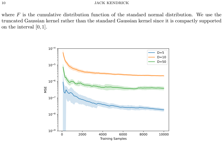
In the Section 5 experiment, the theory predicts that log MSE plotted against log $n$ has slope $-4/(d+4) = -4/7$ for $d=3$; a slope measurably different from this would contradict Theorem 1.2's rate. For Theorem 1.1's premise, one can test Assumption A.2 directly on a rectifiable curve whose tangent angle oscillates non-polynomially in scale, for instance like $1/|\log h|$, and check whether the bias in Lemma 3.1 is truly $O(h^m)$ for some fixed $m$.
Extended reading notes
Core claim
The central claim is Theorem 1.1: for a $d$-rectifiable set $\Omega \subset \mathbb{R}^D$ carrying a probability measure with density $p$ with respect to $H^d$, the estimator $\hat{p}_n(x) = \frac{1}{h_n^d} \sum_{i=1}^n K(\|X_i - x\|/h_n)$ satisfies $\mathrm{MSE}[\hat{p}_n(x)] = O(n^{-2m/(d+2m)})$ with probability one, provided the approximate tangent spaces of $\Omega$ approximate the blow-ups at polynomial rate $O(h^m)$ (Assumption A.2). Theorem 1.2 specializes to sets that are locally smooth manifolds almost everywhere, where the tangent approximation error is $O(h^2)$ by a Taylor expansion, yielding the classical rate $O(n^{-4/(d+4)})$; Whitney stratification shows every $d$-dimensional algebraic variety and semi-algebraic set falls into this class. The proof is the standard bias-variance split: the tangency assumption bounds the bias by $O(h^m)$, variance is $O(1/(n h^d))$, and $h_n \propto n^{-1/(d+2m)}$ balances the two.
Load-bearing premise
The entire rate rests on the unverified exponent $m$ in Assumption A.2: the set's scaled-up neighborhood must approach its tangent plane with error $O(h^m)$, but ordinary rectifiability guarantees only that the error goes to zero, not that it does so polynomially, and the paper gives no way to compute $m$ for a general non-smooth set.
Editorial extensions
If this is right
- On algebraic varieties and semi-algebraic sets, including sparse vectors, low-rank matrices, and positive semidefinite matrices, density estimates converge at $O(n^{-4/(d+4)})$ with no dependence on the ambient dimension $D$.
- The bandwidth choice $h_n \propto n^{-1/(d+4)}$, familiar from manifold density estimation, remains the right scaling for these non-manifold spaces.
- When the set is merely rectifiable without a tangency rate, the estimator is still consistent but no convergence speed is available.
- The method does not require local parametrizations or exponential maps, so it applies on spaces where manifold chart arguments break down.
Reading between the lines
- Because the paper gives no bound on $m$ for a non-smooth rectifiable set, the practical content of Theorem 1.1 depends on a future geometric analysis of tangency rates; for many fractal-like rectifiable sets the rate may fail to be polynomial.
- The theorem only guarantees convergence at $H^d$-almost every point, so behaviour at singular points such as the origin in the sparse-vector variety is open; a pointwise analysis there could require boundary-aware kernels.
- The bias term is $O(h^m)$ and variance is $O(1/(n h^d))$, so the optimal bandwidth could in principle be selected by estimating $d$ and $m$ from data, turning this into an adaptive procedure.
Editorial analysis
A structured set of objections, weighed in public.
Referee Report
Summary. The paper studies the kernel density estimator \hat p_n(x) = (1/(n h_n^d)) \sum_i K(||X_i-x||/h_n) for probability measures supported on a d-rectifiable set \Omega \subset R^D. Under a quantitative tangent-approximation assumption (A.2) that postulates an O(h^m) error in the blow-up integrals of K and K^2, Section 3 derives the bias-variance bound MSE[\hat p_n(x)] = O(h^{2m}) + O(1/(n h^d)), leading to the rate O(n^{-2m/(d+2m)}) for h_n \asymp n^{-1/(d+2m)}. Section 4 proves that on sets that are smooth H^d-almost everywhere the exponent m=2 holds, yielding the classical rate O(n^{-4/(d+4)}) and covering algebraic varieties and semi-algebraic sets. Section 5 reports a numerical experiment for d-sparse vectors in ambient dimensions 5, 10, and 50. The main result is sound only as a conditional theorem; the unconditional statement of Theorem 1.1 is not justified.
Significance. The conditional rate result is a clean and useful generalization of manifold KDE: it separates the geometry of the domain (the tangent approximation exponent m) from the usual bias-variance tradeoff, and Theorem 1.2 gives a short proof of the classical rate for almost-everywhere-smooth sets without reach or exponential-map assumptions. The paper also correctly identifies algebraic varieties and semi-algebraic sets as natural examples. However, the central theorem as stated overclaims: for general rectifiable sets no positive m need exist, so the rate is not a theorem about all rectifiable sets. The fix is local (restate Theorem 1.1 and the abstract conditionally on A.2), and the remaining issues are proofread-level, so the contribution is viable after a major revision.
major comments (2)
- [Section 1, Theorem 1.1; Section 3, Assumption A.2] The theorem is stated for every d-rectifiable set, but the proof relies on Assumption A.2, which postulates a fixed exponent m>0 with O(h^m) in the blow-up integral (6). Rectifiability (Theorem 2.3) guarantees only the limit h to 0, not any polynomial rate. There exist d-rectifiable sets (for example, C^1 curves whose tangent direction has logarithmic modulus of continuity on a fat Cantor set) for which the error in (6) is not O(h^m) for any m>0, so the asserted rate in Theorem 1.1 is false as stated. The formal theorem and the abstract must be restated conditionally: if A.2 holds for some m>0, then the rate holds; without A.2, only consistency is claimed (as the text itself notes in Section 3).
- [Section 4, Lemma 4.1] The Jacobian expansion in the proof is incorrect. Since phi(0)=0 and D phi(0)=0, the Taylor expansion gives D phi(hz)=h D^2 phi(0)(z)+O(h^2), so the lower block of D psi_h is O(h), not O(h^2). Consequently D psi_h(z)^T D psi_h(z)=Id+h^2(D^2 phi(0)(z))^T(D^2 phi(0)(z))+O(h^3), and J_h(z)=1+O(h^2), not 1+O(h^4). The displayed equalities in the proof involving h^4 and (D phi(0)(z))^T(D phi(0)(z)) are false. The lemma's final O(h^2) conclusion still survives because the true O(h^2) Jacobian correction is compatible with the stated error, but the proof must be corrected.
minor comments (6)
- [Section 3, bias-variance decomposition] The displayed decomposition is misprinted; it should read MSE[\hat p_n(x)] = E[(\hat p_n(x)-p(x))^2] = (E[\hat p_n(x)]-p(x))^2 + E[(\hat p_n(x)-E[\hat p_n(x)])^2].
- [Lemmas 3.1 and 3.2] Several integrals over Omega use dP(y) where p(y) dH^d(y) is meant (for example 'p(y)dP(y)' in Lemma 3.1 and Lemma 3.2); since P has density p with respect to H^d, the dP should be dH^d in those lines.
- [Theorems 1.1 and 1.2] The phrase 'with probability 1' following the deterministic MSE bound is not meaningful; the intended statement is presumably 'for H^d-almost every x'.
- [Section 5, kernel formula] The displayed truncated Gaussian kernel is not the kernel used in the paper's estimator: it contains a factor 1/h inside K, and its normalizing constant is the one-dimensional Gaussian CDF, so the integral of K over R^d is not 1 for d=3. Please give the correctly normalized d-dimensional kernel actually used in the code.
- [Section 5, D=50 experiment] With d=3 and n at most 10,000, the expected number of samples in a given coordinate 3-plane is n / binom(50,3) approximately 0.51, so the reported small MSE requires an explanation of the test-point selection and how the estimator is evaluated when no sample lies near the test point.
- [Throughout] There are several typos that should be corrected, including 'Suppse', 'denstiy', 'Coordiante', 'outisde', 'interecting', and 'to to'.
Circularity Check
No significant circularity: the rate claims are explicit consequences of the stated tangent-approximation assumption A.2 and external geometric results.
full rationale
The paper's main rate result, Theorem 1.1, is derived transparently from Assumption A.2, which postulates a polynomial O(h^m) error in the blow-up approximation of the rectifiable set by approximate tangent spaces. The bias estimate in Lemma 3.1 is exactly Assumption A.2 applied to the kernel K, and the variance estimate in Lemma 3.2 is a standard calculation. The bandwidth is then chosen to balance these two terms, giving MSE = O(h^{2m} + 1/(nh^d)) and hence O(n^{-2m/(d+2m)}). The exponent m is an assumed structural parameter, not fitted to the target rate or to the data; the theorem is therefore conditional rather than circular. Theorem 1.2 independently verifies m=2 for almost-everywhere smooth sets using a geometric tangent approximation lemma (Lemma 4.1), whose conclusion is justified by Taylor expansion, not by assuming the desired density-estimation rate. The only citation used as a mathematical foundation is Simon's standard theorem characterizing rectifiable sets via approximate tangent spaces, and Whitney's stratification theorem for algebraic and semi-algebraic sets; neither is a self-citation. The numerical experiment is illustrative and does not serve as evidence for the theorem, so there is no fitted-input-called-prediction issue. The skeptic's concern that Theorem 1.1 as stated omits Assumption A.2, and that not every rectifiable set satisfies A.2 for some m>0, is a correctness and rigor issue about an unstated hypothesis, not a circularity issue. The paper's own text even says the assumption is 'necessary to quantify the rate at which the mean squared error converges,' which is an honest statement of a hypothesis, not a disguised restatement of the conclusion.
Assumptions & free parameters
assumptions (5)
- standard math Kernel K is continuous, vanishes outside [0,1], and satisfies ∫_{R^d} K(||u||) du = 1.
- domain assumption Ω is d-rectifiable and its approximate tangent spaces with respect to p satisfy the O(h^m) convergence in Eq. (6) for the kernel functions used.
- domain assumption The probability P has a density p with respect to H^d on Ω.
- domain assumption For Theorem 1.2, K is twice differentiable, p is twice differentiable, and Ω is locally a smooth (C^3) manifold almost everywhere.
- standard math Algebraic varieties and semi-algebraic sets admit Whitney stratifications and are d-rectifiable.
Cite this review
Pith. "Pith review of Density Estimation on Rectifiable Sets." pith.science (2026). https://pith.science/paper/AYEQC5XV
@misc{pith2026250523023,
  author       = {Pith},
  title        = {Pith review of: Density Estimation on Rectifiable Sets},
  year         = {2026},
  howpublished = {\url{https://pith.science/paper/AYEQC5XV}},
  note         = {Machine review of arXiv:2505.23023}
}
abstract
Kernel density estimation is a popular method for estimating unseen probability distributions. However, the convergence of these classical estimators to the true density slows down in high dimensions. Moreover, they do not define meaningful probability distributions when the intrinsic dimension of data is much smaller than its ambient dimension. We build on previous work on density estimation on manifolds to show that a modified kernel density estimator converges to the true density on $d-$rectifiable sets. As a special case, we consider algebraic varieties and semi-algebraic sets and prove a convergence rate in this setting. We conclude the paper with a numerical experiment illustrating the convergence of this estimator on sparse data.
Figures
Reference graph
Works this paper leans on
-
[6]
Nonparametric estimation of a probability density on a Riemannian manifold using Fourier expansions
url: https://doi.org/10.1016/j.acha.2006.04.006. [Hen90] Harrie Hendriks. “Nonparametric estimation of a probability density on a Riemannian manifold using Fourier expansions”. In:Ann. Statist.18.2 (1990), pp. 832–849.issn: 0090- 5364,2168-8966. doi: 10.1214/aos/1176347628. url: https://doi.org/10.1214/aos/ 1176347628. [KP13] Yoon Tae Kim and Hyun Suk Par...
arXiv 1990
-
[2020]
Density estimation on an unknown submanifold
arXiv: 1910.08477 [math.ST]. url: https://arxiv.org/abs/1910.08477. [BS17] Tyrus Berry and Timothy Sauer. “Density estimation on manifolds with boundary”. In: Comput. Statist. Data Anal.107 (2017), pp. 1–17. issn: 0167-9473,1872-7352. doi: 10. 1016/j.csda.2016.09.011. url: https://doi.org/10.1016/j.csda.2016.09.011. [Cac66] Theophilos Cacoullos. “Estimati...
work page Pith review arXiv 2017
Reviewed August 7, 2026 · model on record in the stance chip above.
Discussion (0). Continue with ORCID to comment.