REVIEW 5 major objections 6 minor 40 references
A Probabilistic Representation of Deep Learning
T0 review · 5 major / 6 minor · reviewed 2026-08-14 · deepseek-v4-flash
Pith's one-line read A deep neural network is a Bayesian hierarchical model whose layers are Gibbs distributions, with early layers forming a prior and later layers a likelihood, this paper claims.
desk verdict The paper's central generalization claim is undercut by a wrong KL decomposition, and the Gibbs representation is a post-hoc definition rather than a derivation. read the letter →
The pith
A machine-rendered reading of the paper's core claim, the machinery that carries it, and where it could break.
The reading
What carries the argument
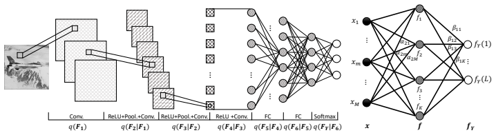
The carrying machinery is the Markov-chain factorization $q(F_1;\ldots;F_I;F_Y)=q(F_1)\prod_{i=1}^{I-1}q(F_{i+1}|F_i)q(F_Y|F_I)$, combined with the neuron-as-energy mapping $E_F(k)=-g_k(x)$, which turns any hidden layer into a Gibbs distribution $p(F_k)=\exp\{g_k(x)\}/Z$. The softmax output is the same construction over label configurations, and known results identify convolutional-plus-nonlinear blocks with Markov random fields, another Gibbs family. Because an energy function is a sufficient statistic for a Gibbs distribution, defining the layer's energy is taken to define the layer's distribution; because the chain product is a Bayesian hierarchical model, the network splits into a prior part and a likelihood part. Conjugacy of Gibbs distributions and the backward flow of backpropagation are the mechanism said to let the prior be inferred indirectly through the likelihood.
What would settle it
On a trained network from the paper's synthetic dataset, compute both sides of the claimed identity $KL[p_\theta(Y,X)||q(Y,X)] = KL[p(Y|X)||q(Y|X)] + KL[p(X)||q(X)]$: if the two sides differ because the right-hand side omits an expectation over $X$, the decomposition used to blame backpropagation is not an equality. A second check is to add an explicit input-prior matching term to the loss and see whether generalization improves as the argument predicts.
Extended reading notes
Core claim
On the paper's account, a deep neural network is a probabilistic model in a literal sense. The forward pass is a Markov chain $F_1\to\cdots\to F_I\to F_Y$, so the joint distribution factorizes as $q(F_1)q(F_2|F_1)\cdots q(F_Y|F_I)$. Each neuron $g_k(x)$ is treated as the negative energy of a Gibbs distribution, making each hidden layer a Gibbs distribution via its energy function, and the softmax output is a discrete Gibbs distribution over labels. Proposition 1 states that the whole architecture is therefore a Bayesian hierarchical model, and Proposition 2 states that hidden layers formulate Gibbs distributions. The hierarchy is a split between layers modeling a prior $q(X)$ and layers modeling a likelihood $q(Y|X)$. The generalization claim is that learning $q(X)$ is an explicit regularizer, while the standard relaxed loss—viewed as variational inference—optimizes only the label-conditional divergence, so the prior is learned only indirectly and can be a poor match to $p(X)$; this is offered as the reason backpropagation can reduce generalization, and as the explanation for why over-parametrized networks still generalize and why random labels give chance-level test error. Experiments on a synthetic Gaussian-distributed digit dataset show the first-layer energy histogram close to $p(X)$ and are offered as validation.
Load-bearing premise
The argument stands on the assumption that the training objective separates exactly into a term for getting the labels right and a term for matching the input distribution; if that separation is not an equality—say, because the input-distribution term must be weighted by the data distribution inside an expectation—then the conclusion that backpropagation limits generalization by ignoring the input prior does not follow.
Editorial extensions
If this is right
- If the representation is correct, over-parametrization is not inherently dangerous: extra hidden units can improve the learned prior $q(X)$, which regularizes the likelihood, so larger networks can generalize better rather than overfit.
- Standard backpropagation is an incomplete variational inference: it fits the likelihood term of the divergence and leaves the prior term unoptimized, which predicts that two networks with identical prior-layer formulas but different later layers will learn different priors, exactly the CNN1 versus CNN2 comparison in the paper.
- Random-label experiments are consistent with generalization: the network still learns a good $q(X)$ and can always find some feature separating the training labels, but since the true labels are independent of $X$, test error stays at chance.
- The hierarchy property gives a principled way to say which part of a network is doing prior modeling and which part is doing likelihood modeling, so layer-wise transfer or feature-extraction decisions can be guided by the probabilistic role of each layer.
Reading between the lines
- A direct testable extension is to add an explicit prior-matching penalty to the relaxed loss, such as a divergence between the early-layer feature distribution and an estimate of $p(X)$; the representation predicts this should improve generalization, though the paper does not run that experiment.
- The energy-function representation makes layer densities explicit enough that information-theoretic quantities like mutual information between layers become computable from trained weights, which could connect this hierarchy picture to information-bottleneck analyses without altering the network.
- The prior-likelihood split suggests a design rule the paper does not state: architectures that put more capacity in early layers should generalize better on small or noisy datasets, because that is where the regularizing prior is learned.
Signed reviews
Editorial analysis
A structured set of objections, weighed in public.
Referee Report
Summary. The paper proposes a probabilistic representation of deep neural networks in which each neuron defines an energy function of a Gibbs distribution, each hidden layer is said to formulate a Gibbs distribution, and the whole network is interpreted as a Bayesian hierarchical model. On this basis, the authors argue that the hierarchy of DNNs corresponds to a split into a learned prior q(X) and a likelihood q(Y|X), that DNNs perform explicit regularization by learning q(X), and that the relaxed training loss used by backpropagation fails to infer q(X) and therefore limits generalization. The claims are supported by KL divergence calculations on a synthetic Gaussian pixel dataset and by experiments on over-parametrization and random labels.
Significance. If the proposed representation were correct, it would offer a unified energy-based and Bayesian view of DNN architecture and could connect regularization to learning the input distribution. The paper is clearly written, the synthetic setup is simple, and the idea of treating early layers as learning a data-dependent prior is intuitively appealing. However, the central steps are either definitional or mathematically incorrect: the Gibbs-distribution claim in Proposition 2 imposes no constraints because any neuron output can be normalized into a distribution, and the generalization argument in Section 4.2 uses an incorrect KL decomposition. The experimental validation compares distributions on different spaces and therefore cannot corroborate the representation. As a result, the claimed explanatory power is not established.
major comments (5)
- [Section 3, Proposition 2 and Eq. (7)] The construction p(F_k)=exp(g_k(x))/Z_F with energy E_F(k)=-g_k(x) defines a normalized distribution over the neuron index k for any function g_k, so every deterministic layer, trained or untrained, trivially admits this representation. The text itself concedes that hidden layers only formulate the corresponding energy functions, rather than directly formulating Gibbs distributions; since any finite energy function defines a Gibbs distribution after normalization, Proposition 2 is true by construction and imposes no testable constraint. Similarly, the Markov factorization in Eq. (5) holds for any feedforward network, and the conditional distributions q(F_i|F_{i-1}) are degenerate for deterministic layers, so calling the network a Bayesian hierarchical model is a relabeling rather than a derived result. This definitional step cannot support the subsequent explanation of generalization.
- [Section 4.2, KL decomposition before Eq. (13)] The identity KL[p_theta(Y,X)||q(Y,X)] = KL[p(Y|X)||q(Y|X)] + KL[p(X)||q(X)] is mathematically incorrect. The chain rule for KL divergence is KL[p(x,y)||q(x,y)] = KL[p(x)||q(x)] + E_{p(x)} KL[p(y|x)||q(y|x)]. The missing expectation over X is load-bearing: without it, the conclusion that the relaxed loss merely corresponds to KL[p(Y|X)||q(Y|X)] and therefore ignores q(X) does not follow. This invalidates the paper's central claim that backpropagation is a reason for decreasing the generalization ability of DNNs.
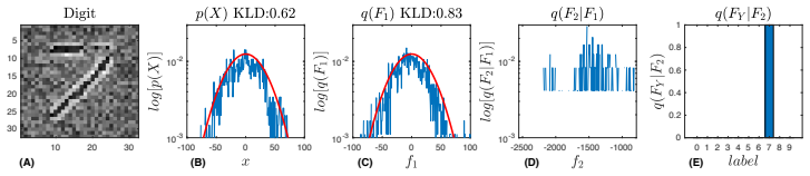
- [Section 5.1, Figure 3 and Section 5.2.1] The reported KL divergences compare incompatible objects. p(X)=N(0,1024) is a distribution over pixel intensities or pixel vectors, while q(F1) is estimated by a histogram of the scalar energy E_{F1}; these are distributions of different random variables, so KL[p(X)||q(F1)] is not a well-defined measure of how well f1 models p(X). The same problem affects KL[p(X)||qCNN1(F1)]=0.94 and =1.59 in Section 5.2.1 and =0.60 in Section 5.2.2. Additionally, using the histogram of a one-dimensional energy to represent the full joint distribution q(F1) is unjustified; sufficiency of the energy for the Gibbs family does not imply that its marginal histogram determines the layer's full distribution.
- [Section 5.2.2, random labels argument] The claim that a DNN cannot model random labels because q(X,Y)=q(Y|X)q(X) only models dependent variables is false: q(Y|X) can be chosen independent of X, giving q(X,Y)=q(Y)q(X), so the model class can represent independence. The toy example is also not an instance of random labels, since it posits that the labels are a deterministic function of the 'full' feature that the DNN detects. This weakens the paper's clarification of the random-label phenomenon.
- [Section 4.1 and Section 5.1, prior/likelihood split] The division of layers into prior and likelihood is post hoc. The paper states there is no clear boundary, and in Section 5.1 f1 is designated the prior because max pooling compresses too much information; this criterion is not derived from the probabilistic representation. Because the split can be chosen after training to fit the data, the hierarchy claim is unfalsifiable and cannot serve as an explanation of DNN hierarchy.
minor comments (6)
- [Throughout] The phrases 'the truly posterior distribution' and 'the truly prior distribution' should be 'the true posterior distribution' and 'the true prior distribution'.
- [Section 5.1] 'perspective histograms' should be 'respective histograms'.
- [Equation (6)] The expression for Z' is ambiguous in the text; it should be typeset as Z' = Z / prod_k Z_F^{beta_{lk}}.
- [Figure 3 caption] The notation KL[p(X)||p(x)] uses p for both the population distribution and the empirical histogram of a single image, which is confusing; please use distinct symbols.
- [Section 5.2.1] Calling CNN1 and CNN2 over-parametrized because they have 1680 and 1330 parameters while an image has 1024 pixels is nonstandard; over-parametrization usually refers to capacity relative to the number of training examples, so the term should be clarified.
- [Section 5] The experimental section does not specify how histograms are constructed or how the KL divergences are computed (bin width, support, normalization), which makes the quantitative claims difficult to reproduce.
Circularity Check
The probabilistic representation is constructed rather than derived: Eq. (7) turns any neuron output into a Gibbs distribution by defining its energy, Eqs. (4)-(5) rename the chain-rule factorization as a Bayesian hierarchical model, and the generalization argument rests on a misstated KL decomposition.
-
self definitional
[Section 3, Proposition 2, Eqs. (6)-(7)]
"It is noteworthy that all experts p(F ) = {p(Fk)}K k=1 are Gibbs distributions expressed as p(Fk) = 1/ZF exp{gk(x)}, (7) where the energy function is equivalent to the negative of the kth neuron, i.e., EF (k) = −gk(x)."
Equation (7) constructs the Gibbs distribution from an arbitrary neuron output g_k(x) by setting its energy to -g_k(x). Therefore every deterministic hidden layer, trained or untrained, automatically 'formulates' a Gibbs distribution; the proposition is an ansatz/definition, not a derived property of DNNs. The paper itself concedes this: 'hidden layers only formulate the corresponding energy functions, rather than directly formulating Gibbs distributions.' No constraint is imposed, so the later claim that this explains regularization/generalization is a relabeling of the construction.
-
renaming known result
[Section 3, Proposition 1, Eqs. (4)-(5)]
"Since the input of the hidden layer fi in the DNN = {x;f1;...;fI ;fY} is the output of its previous layer fi−1, we can derive that the DNN = {x;f1;...;fI ;fY} forms a Markov chain as F1→···→ FI→FY. (4) As a result, the distribution of the DNN can be formulated as q(F1;...;FI ;FY ) = q(F1)·...q(Fi+1|Fi)·...q(FY|FI )."
The stated factorization is the chain rule applied to any sequence of random variables; any feed-forward network, indeed any set of variables ordered in a chain, satisfies it. Calling this a 'Bayesian hierarchical model' renames the universally valid product rule rather than deriving a property specific to DNNs. The subsequent hierarchy claim (Eq. (10)) then simply designates some factors as 'prior' and others as 'likelihood,' so the 'explicit regularization by learning q(X)' is chosen by labeling, not derived.
full rationale
The central derivation is definitional. Proposition 2 reduces to 'define a Gibbs distribution with energy -neuron output,' which makes the Gibbs claim true by construction for every possible layer and hence carries no explanatory content. Proposition 1 reduces to the chain-rule factorization of an arbitrary joint distribution, renamed as a Bayesian hierarchical model. These two definitions are then used as the premise for the hierarchy and generalization conclusions, so the paper's positive claims about 'explicit regularization' and 'learning a prior q(X)' are imposed by the representational choices rather than established. The Section 4.2 argument additionally contains a mathematical error: the equality KL[pθ(Y,X)||q(Y,X)] = KL[p(Y|X)||q(Y|X)] + KL[p(X)||q(X)] omits the expectation E_{p(X)} in the conditional KL term, so the conclusion that the relaxed loss 'merely corresponds' to the likelihood term and cannot guarantee generalization does not follow from the stated identity. Section 5 does not repair this: it validates the representation by comparing KL[p(X)||q(F1)] where p(X) is the pixel-intensity distribution and q(F1) is estimated from a histogram of the scalar energy E_{F1}, i.e., distributions on different spaces, so the numerical KL values (0.83, 0.94, 1.59) cannot substantiate the claims. No self-citation chain is load-bearing here; the circularity is internal to the definitions. Score 8 reflects that the paper's central representation is forced by construction.
Assumptions & free parameters
free parameters (2)
- synthetic data variance =
1024
- prior/likelihood boundary =
f1 as prior for CNN1/CNN2
assumptions (5)
- ad hoc to paper The KL chain rule holds as KL[pθ(Y,X)||q(Y,X)] = KL[p(Y|X)||q(Y|X)] + KL[p(X)||q(X)] without an expectation.
- domain assumption A hidden layer's energy function is defined as the negative of its neuron outputs, so each hidden layer yields a Gibbs distribution.
- ad hoc to paper The prior/likelihood boundary in the hierarchy is fixed by the modeler and is not ambiguous.
- domain assumption The true posterior p(F1...FI,FY|D) can be expressed as pθ(Y,X).
- domain assumption A trained DNN's activations have a joint distribution that factorizes into conditional Gibbs distributions given the input.
invented entities (2)
-
Gibbs distribution per neuron, p(F_k)=exp(g_k(x))/Z_F
-
Prior distribution q(X) learned by early layers
Cite this review
Pith. "Pith review of A Probabilistic Representation of Deep Learning." pith.science (2026). https://pith.science/paper/B264255I
@misc{pith2026190809772,
  author       = {Pith},
  title        = {Pith review of: A Probabilistic Representation of Deep Learning},
  year         = {2026},
  howpublished = {\url{https://pith.science/paper/B264255I}},
  note         = {Machine review of arXiv:1908.09772}
}
read the original abstract
In this work, we introduce a novel probabilistic representation of deep learning, which provides an explicit explanation for the Deep Neural Networks (DNNs) in three aspects: (i) neurons define the energy of a Gibbs distribution; (ii) the hidden layers of DNNs formulate Gibbs distributions; and (iii) the whole architecture of DNNs can be interpreted as a Bayesian neural network. Based on the proposed probabilistic representation, we investigate two fundamental properties of deep learning: hierarchy and generalization. First, we explicitly formulate the hierarchy property from the Bayesian perspective, namely that some hidden layers formulate a prior distribution and the remaining layers formulate a likelihood distribution. Second, we demonstrate that DNNs have an explicit regularization by learning a prior distribution and the learning algorithm is one reason for decreasing the generalization ability of DNNs. Moreover, we clarify two empirical phenomena of DNNs that cannot be explained by traditional theories of generalization. Simulation results validate the proposed probabilistic representation and the insights into these properties of deep learning based on a synthetic dataset.
Figures

Figures from the paper (3 more)


Reference graph
Works this paper leans on
-
[1]
Alessandro Achille and Stefano Soatto. Emergence of invariance and dis- entanglement in deep representations.arXiv preprint arXiv:1706.01350, 2017
arXiv 2017
-
[2]
Nearly-tight VC-dimension and pseudodimension bounds for piecewise linear neural networks
Peter L. Bartlett, Nick Harvey, Christopher Liaw, and Abbas Mehrabian. Nearly-tight vc-dimension and pseudodimension bounds for piecewise linear neural networks.arXiv preprint arXiv:1703.02930, 2017
work page Pith review arXiv 2017
-
[3]
Representation learning: A review and new perspectives.IEEE Transactions on Pattern Analysis and Machine Intelligence, 35(8):1798–1828, 2013
Yoshua Bengio, Aaron Courville, and Pascal Vincent. Representation learning: A review and new perspectives.IEEE Transactions on Pattern Analysis and Machine Intelligence, 35(8):1798–1828, 2013
2013
-
[4]
David Blei, Alp Kucukelbir, and Jon MaAuliffe. Variational inference: A review for statisticians.Journal of Machine Learning Research, 112:859–877, 2017
work page 2017
-
[5]
Stability and generalization.Journal of Machine Learning Research, pages 499–526, 2002
Olivier Bousquet and Andre Elisseeff. Stability and generalization.Journal of Machine Learning Research, pages 499–526, 2002. 13
work page 2002
-
[6]
John Bridle. Training stochastic model recognition algorithms as networks can lead to maximum mutual information estimation of parameters. In NeurIPS, 1990
work page 1990
-
[7]
Pratik Chaudhari and Stefano Soatto. Stochastic gradient descent performs variational inference, converges to limit cycles for deep networks. InITA, 2018
work page 2018
-
[8]
Wiley- Interscience, Hoboken, New Jersy, 2006
Thomas Cover and Joy Thomas.Elements of Information Theory. Wiley- Interscience, Hoboken, New Jersy, 2006
work page 2006
Show all 40 references
-
[9]
Geman and D
S. Geman and D. Geman. Stochastic relaxation, gibbs distributions, and the bayesian restoration of images.IEEE Transactions. on Pattern Analysis and Machine Intelligence, pages 721–741, June 1984
1984
-
[10]
A probabilistic approach to the understanding and training of neural network classifiers
Herbert Gish. A probabilistic approach to the understanding and training of neural network classifiers. InIEEE ICASSP, pages 1361–1364, 1990
1990
-
[11]
MIT Press, 2016
Ian Goodfellow, Yoshua Bengio, and Aaron Courville.Deep Learning. MIT Press, 2016
2016
-
[12]
Lawrence
James Hensman, Magnus Rattray, and Neil D. Lawrence. Fast variational inference in the conjugate exponential family. InNeurIPS, 2012
2012
-
[13]
Geoffrey E. Hinton. Training products of experts by minimizing contrastive divergence. Neural Computation, 14:1771–1800, 2002
2002
-
[14]
Hoffman, David M
Matthew D. Hoffman, David M. Blei, Chong Wang, and John Paisley. Stochastic variational inference. Journal of Machine Learning Research, 14:1303–1347, 2013
2013
-
[15]
MichaelI.Jordan, ZoubinGhahramani, TommiS.Jaakkola, andLawrenceK. Saul. An introduction to variational methods for graphical models.Machine Learning, 37:183–233, 1999
1999
-
[16]
Xinjie Lan and Kenneth E. Barner. From mrfs to cnns: A novel image restoration method. In52nd Annual Conference on Information Sciences and Systems (CISS), pages 1–5, 2018
2018
-
[17]
MIT Press, 2006
Yann LeCun, Sumit Chopra, Raia Hadsell, Marc’Aurelio Ranzato, and Fu Jie Huang.A tutorial on energy-based learning. MIT Press, 2006
2006
-
[18]
A bayesian hierarchical model for learning natural scene categories
Feifei Li and Pietro Perona. A bayesian hierarchical model for learning natural scene categories. InCVPR, 2005
2005
-
[19]
Stan Z. Li. Markov Random Field Modeling in Image Analysis 2nd ed. Springer, New York, 2001
2001
-
[20]
Pankaj Mehta and David J. Schwab. An exact mapping between the variational renormalization group and deep learning. arXiv preprint arXiv:1410.3831, 2014. 14
2014 arXiv
-
[21]
Kevin P. Murphy. Conjugate bayesian analysis of the gaussian distribution. Technical report, University of British Columbia, 2007
2007
-
[22]
Deeplearningandtheinformationbottleneck principle
NogaZaslavskyNaftaliTishby. Deeplearningandtheinformationbottleneck principle. arXiv preprint arXiv:1503.02406, 2015
2015 arXiv
-
[23]
Exploring generalization in deep learning
Behnam Neyshabur, Srinadh Bhojanapalli, David McAllester, and Nathan Srebro. Exploring generalization in deep learning. InNeurIPS, 2017
2017
-
[24]
In search of the real inductive bias: On the role of implicit regularization in deep learning
Behnam Neyshabur, Ryota Tomioka, and Nathan Srebro. In search of the real inductive bias: On the role of implicit regularization in deep learning. In ICLR, 2015
2015
-
[25]
Ng and Michael I
Andrew Y. Ng and Michael I. Jordan. On discriminative vs. generative classifiers: A comparison of logistic regression and naive bayes. InNeurIPS, pages 841–848, 2002
2002
-
[26]
Statistical exponential families: A digest with flash cards.arxiv preprint arXiv:0911.4863, 2011
Frank Nielsen and Vincent Garcia. Statistical exponential families: A digest with flash cards.arxiv preprint arXiv:0911.4863, 2011
2011 arXiv
-
[27]
Aprobabilisticframework for deep learning
AnkitPatel, MinhNguyen, andRichardBaraniuk. Aprobabilisticframework for deep learning. InNeurIPS, 2016
2016
-
[28]
Theoretical impediments to machine learning with seven sparks from the causal revolution.arXiv preprint arXiv:1801.04016, 2018
Judea Pearl. Theoretical impediments to machine learning with seven sparks from the causal revolution.arXiv preprint arXiv:1801.04016, 2018
2018 arXiv
-
[29]
Richard and R.P
M.D. Richard and R.P. Lippmann. Neural network classifiers estimate bayesian a posteriori probabilities. Neural Computation, pages 461–483, 1991
1991
-
[30]
Rumelhart, Geoffrey E
David E. Rumelhart, Geoffrey E. Hinton, and Ronald J. Williams. Learning representations by back-propagating errors.Nature, 323:533–536, October 1986
1986
-
[31]
Deep boltzmann machines
Ruslan Salakhutdinov and Geoffrey Hinton. Deep boltzmann machines. In AISTATS 2009, pages 448–455, 2009
2009
-
[32]
On the information bottleneck theory of deep learning
Andrew Saxe, Yamini Bansal, Joel Dapello, Madhu Advani, Artemy Kolchin- sky, Brendan Tracey, and David Cox. On the information bottleneck theory of deep learning. InICLR, 2018
2018
-
[33]
Opening the black box of deep neural networks via information.arXiv preprint arXiv:1703.00810, 2017
Ravid Shwartz-Ziv and Naftali Tishby. Opening the black box of deep neural networks via information.arXiv preprint arXiv:1703.00810, 2017
2017 arXiv
-
[34]
E. P. Simoncelli. Statistical models for images: Compression, restoration and synthesis. In Proc 31st Asilomar Conf on Signals, Systems and Computers, pages 673–678, November 1997
1997
-
[35]
Jaakkola
Harald Steck and Tommi S. Jaakkola. On the dirichlet prior and bayesian regularization. In NeurIPS, 2003. 15
2003
-
[36]
Deep mixtures of factor analysers.arXiv preprint arXiv:1206.4635, 2015
Yichuan Tang, Ruslan Salakhutdinov, and Geoffrey Hinton. Deep mixtures of factor analysers.arXiv preprint arXiv:1206.4635, 2015
2015 arXiv
-
[37]
Martin. J. Wainwright and Eero. P. Simoncelli. Scale mixtures of gaussians and the statistics of natural images. InNeurIPS, pages 855–861, 2000
2000
-
[38]
Understanding deep learning requires rethinking generalization
Chiyuan Zhang, Samy Bengio, Moritz Hardt, Benjamin Recht, and Oriol Vinyals. Understanding deep learning requires rethinking generalization. In ICLR, 2016
2016
-
[39]
G. Zhang. Neural networks for classification: a survey.IEEE Transactions on Systems, Man, and Cybernetics, 30:451–462, 2000
2000
-
[40]
Conditional random fields as recurrent neural networks
Shuai Zheng, Sadeep Jayasumana, Bernardino Romera-Paredes, Vibhav Vineet, ZhizhongSu, DalongDu, ChangHuang, andPhilipTorr. Conditional random fields as recurrent neural networks. InInternational Conference on Computer Vision (ICCV), pages 1529–1537, 2015. 16
2015
Reviewed August 14, 2026 · model on record in the stance chip above.
Discussion (0). Continue with ORCID to comment.