REVIEW 4 major objections 5 minor 31 references
Reconstruction of the observable universe from the integrated Sachs-Wolfe effect
T0 review · 4 major / 5 minor · reviewed 2026-08-06 · deepseek-v4-flash
Pith's one-line read This paper proves that initial gravitational perturbations in a shell around the last-scattering surface can be stably recovered from integrated Sachs-Wolfe observations made near the observer.
desk verdict Partial-data ISW tomography with real microlocal content, but Lemma 5.1 has a gap that leaves Theorem 2.1 unproved as written. read the letter →
The pith
A machine-rendered reading of the paper's core claim, the machinery that carries it, and where it could break.
The reading
What carries the argument
The load-bearing construction is the microlocal analysis of the backprojection of the light ray transform. The paper uses a modified transform $L_\epsilon = \varphi_\epsilon L$ with cutoff $\varphi_\epsilon$ supported in $B_{1-\epsilon}$ to avoid boundary artifacts, and two backprojections: $I h(x)=\int_{S^2} h(x,v)\,dv$ and a weighted version $I^\varphi h(x)=\int_{S^2}\varphi(v)h(x,v)\,dv$ with $\varphi$ chosen so that $\varphi(\xi/|\xi|)\neq \varphi(-\xi/|\xi|)$. Stationary phase decomposes $I L_\epsilon E^\pm_j$ into Fourier integral operators with canonical relations $C_a = \{(x,\xi;y,\eta): \xi=\eta,\ x=y-a\xi/|\xi|\}$; combining the two backprojections cancels the leading-order terms and yields, via parametrices $Q^\pm, W^\pm, S$, explicit inversion formulas for $f_2$ and $f_1$ modulo regularizing operators.
What would settle it
Run the paper's numerical discretization on initial data supported in the shell $R_{T-1,T+1}$ for a small detector grid such as $7\times7$ and inspect the singular values of the forward matrix restricted to that subspace; singular values at machine precision would indicate a nontrivial numerical null space, contradicting the claimed stability. Alternatively, attempt to construct nonzero compactly supported $(f_1,f_2)$ in the shell whose wave solution satisfies $Lu=0$ on $B\times S^2$; any such pair directly refutes Theorem 2.1.
Extended reading notes
Core claim
On its own terms, the paper proves a stability estimate for the cosmological X-ray transform with partial data. For the wave equation $P u=0$ with $P = \Box + a_0 \partial_t + \sum a_j D_j + b$, Theorem 2.1 states that if $f_1 \in H^{s+1}(\mathbb{R}^3)$ and $f_2 \in H^s(\mathbb{R}^3)$ are compactly supported in the spherical shell $R_{T-1,T+1}$, then the observations $Lu$ on $B \times S^2$ determine $f_1, f_2$ uniquely and $$\|f_1\|_{$H^{{s+1}}$} + \|f_2\|_{H^s} \leq C \|Lu\|_{$H^{{s+2}}$},$$ with $C$ uniform over data supported in a fixed compact subset of the shell. This is the first stable recovery result for the ISW problem in the realistic setting where observations are confined to a small region near the Earth rather than a full Cauchy surface. The paper also constructs an explicit microlocal inversion, formulas (4.16) and (4.17), that recovers $f_2$ and then $f_1$ up to smoother terms, and it reports two-dimensional numerical reconstructions showing the shell structure emerging from simulated noisy ISW data.
Load-bearing premise
The proof's load-bearing premise is the unproved unique-continuation step that $Lu=0$ forces the initial data supported in the shell $R_{T-1,T+1}$ to vanish; if that implication fails, the compactness argument collapses and the stability estimate may only hold modulo smoother terms.
Editorial extensions
If this is right
- Initial data in the shell $R_{T-1,T+1}$ can be recovered with a quantified loss of three Sobolev derivatives: data in $H^{s+1}\times H^s$ are controlled by observations in $H^{s+2}$.
- The stability estimate is uniform over compact families of data, so small metric perturbations of the background can be handled by the same argument.
- In the partial-data regime the discrete forward problem is severely ill-posed, with condition numbers growing rapidly as the detector grid shrinks, so regularization is essential; the paper's experiments with sparsity and edge-preserving priors demonstrate this.
- The microlocal inversion formulas can in principle characterize which wave-front directions of data supported in the full ball $B_{T+1}$ are recoverable, extending the result beyond the shell.
Reading between the lines
- Editorial inference: the same stationary-phase decomposition should yield a precise visible wave-front set for data supported in the whole ball $B_{T+1}$; writing it out would turn the remark after Theorem 2.1 into a full microlocal uniqueness theorem.
- Editorial inference: the physical model, not the ray transform alone, is what stabilizes the inversion; this suggests that other causal PDE constraints, such as sound-speed wave equations for fluids, could stabilize otherwise ill-posed ISW inversions similarly.
- Editorial inference: the unproved unique-continuation step could be tested numerically by computing the singular value spectrum of the discretized forward operator restricted to shell-supported initial data; a nontrivial numerical null space would indicate the stability estimate needs modification.
Signed reviews
Editorial analysis
A structured set of objections, weighed in public.
Referee Report
Summary. The paper studies the inverse problem of recovering the initial Cauchy data (f1,f2) of a scalar perturbation solving a wave equation with lower-order terms from the light ray transform Lu of the solution, where the transform is observed on a unit ball at the final time t=T. The main result, Theorem 2.1, claims stable and unique recovery of data supported in the shell R_{T-1,T+1}, with the H^{s+2} norm of Lu controlling the H^{s+1} and H^s norms of f1 and f2. The proof combines a microlocal inversion based on backprojection (Sections 3-4) with a compactness argument (Section 5) that requires a uniqueness lemma for the light ray transform. The paper also contains a numerical study for a 2D model comparing several regularization approaches.
Significance. If Theorem 2.1 were fully established, the paper would be a significant contribution to cosmological X-ray tomography: it would provide a parameter-free stability estimate for partial-data recovery from the integrated Sachs-Wolfe effect, extending the full-data results of Vasy and Wang. The microlocal construction in Sections 3-4 is substantial and plausible, and the numerical experiments with synthetic data illustrate the potential of regularized inversion. However, the central stability theorem currently rests on a uniqueness lemma that is false as stated and whose proof is invalid, so the significance is conditional on repairing the uniqueness argument.
major comments (4)
- [Section 5, Lemma 5.1] The lemma as stated is false for arbitrary u in H^s. Take u(t,x)=a(t) with a in C_c^∞(0,T) and ∫_0^T a(t)dt=0; then Lu(y,v)=0 for all (y,v), but u is not zero on the set (5.2). Moreover, the proof does not establish the stated conclusion: in (5.3), the function A(t,x)=χ(t)φ(x−tv+Tv)u(t,x) depends on v, so the identity \hat A_v(−v·ξ,ξ)=0 is for a different function for each v. An entire function can vanish on the hyperplane τ=−v·ξ without being identically zero, and the union of these hyperplanes over v does not give a fixed analytic function vanishing on an open set. Thus the claim u=0 on (5.2) is not proved.
- [Section 5, Eq. (5.2)] The displayed visibility region is incorrect. A point (t,x) lies on a null ray through B at time T exactly when there exists v∈S² with |x−(t−T)v|<1, i.e., when T−t−1<|x|<T−t+1 (for T−t>1). The region T−t≤|x|<T−t+1 in (5.2) omits the inner shell T−t−1<|x|<T−t. At t=0 this means the lemma would only constrain T≤|x|<T+1, not the full support R_{T−1,T+1} of the data in Theorem 2.1, so the contradiction argument cannot force f1=f2=0.
- [Section 5, proof of Theorem 2.1] The passage from the a priori estimate (5.1) to the final estimate (2.5) depends entirely on removing the terms C∥f1∥_{H^s}+C∥f2∥_{H^{s−1}} by the compactness argument. Since that removal uses Lemma 5.1, and the lemma is neither true as stated nor proved for solutions of (2.4), the central stability estimate is not established. The proof must supply a valid unique continuation result for solutions of the wave equation with lower-order terms, or replace the compactness argument.
- [Section 3, Eqs. (3.7)-(3.8)] The stationary-phase assignments appear to be interchanged for the E+ contribution. The critical point v=+ξ/|ξ| yields the phase (x−y)·ξ+(2t−T−ϵ)|ξ|, while v=−ξ/|ξ| yields (x−y)·ξ+(T+ϵ)|ξ|; in (3.7) the phase factors e^{i(T+ϵ)|ξ|} and e^{-i(T+ϵ)|ξ|}e^{i2t|ξ|} are assigned to b+_{1,1} and b+_{1,2} respectively, while the symbols in (3.8) use the opposite arguments ±ξ/|ξ|. This inconsistency should be resolved, since the canonical relations and principal symbols from Lemma 3.1 feed into the parametrix construction in Section 4.
minor comments (5)
- [Section 2, Theorem 2.1] The paper should state the assumption T>1, or explicitly invoke the convention R_{a,b}=B_b for a≤0, because the proof selects ϵ with the support contained in R_{T−1+2ϵ,T+1−2ϵ}.
- [Section 4, Eqs. (4.10)-(4.14)] There are apparent typos in the parametrix definitions; for example W+ is introduced as a parametrix of the f2 coefficient but is then used to isolate f1, and (4.11) appears to isolate f1 instead of f2. These need to be corrected and checked.
- [Section 5, Lemma 5.1] If the intended uniqueness statement is only for solutions of (2.4), the lemma should say so and the proof must use the equation; the present proof never uses it, and the counterexample in my major comment shows the unrestricted statement is false.
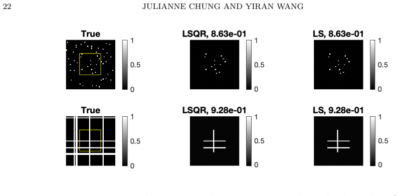
- [Section 6] The numerical experiments solve a 2D discrete inverse problem and do not directly validate the 3D stability estimate (2.5); the conclusions in Section 7 should describe the numerics as heuristic support rather than as a demonstration of Theorem 2.1.
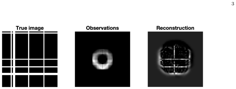
- [Figure 1] The caption refers to visible structures 'in the region given by Theorem 2.1' for a 2D example; since the theorem is stated for R^3, the caption should clarify the relation.
Circularity Check
No significant circularity: the new partial-data theorem is proved by the paper's own microlocal inversion and compactness argument; prior self-citations are motivational or technical, not load-bearing.
full rationale
The central claim (Theorem 2.1) is not equivalent by construction to any of its inputs. The derivation starts from the forward transform (2.2), decomposes the backprojections into Fourier integral operators (Lemmas 3.1 and 3.2, and the analogous weighted versions in Section 4), then solves for f1 and f2 modulo regularizing terms through the parametrices leading to (4.16)-(4.17). The lower-order terms are removed in Section 5 by a compactness argument that uses the separate uniqueness statement of Lemma 5.1; even if that lemma has a mathematical gap, its use is not circular because Lemma 5.1 is not obtained from the theorem being proved. The cited prior work by the authors ([28], [30], [31], [5]) provides background, the backprojection approach, and a numerical discretization, but no load-bearing theorem is imported from those papers; the parametrices and estimates are constructed in this paper. Lemmas 4.1 and 4.2 are explicitly stated with proofs omitted, which is a completeness gap rather than a circularity, since the asserted decompositions are direct analogues of Lemmas 3.1-3.2 and are not derived from the theorem's conclusion. The numerical study is a synthetic test against known phantom images, with no fitted parameter being relabeled as a prediction. No circular step satisfying the quote-and-reduction standard was found.
Assumptions & free parameters
assumptions (6)
- standard math Hormander FIO calculus: graph FIO composition, Sobolev mapping properties, elliptic parametrices exist.
- standard math Oscillatory integral representation of solutions to (2.3) with elliptic amplitudes (Treves).
- standard math Well-posedness and energy estimates for the Cauchy problem (2.4) with smooth coefficients.
- domain assumption Linearized cosmology: scalar-field perturbation Phi satisfies the damped wave equation (1.2), and the ISW effect is proportional to the integral of d_s Phi along null geodesics.
- domain assumption Observation geometry: detectors fill a unit ball B at t=T, all directions v in S^2 are observed, and initial data are supported in the shell R_{T-1,T+1}.
- ad hoc to paper Unique continuation: if a solution u of (2.4) vanishes on S (5.2), then the Cauchy data supported in R_{T-1,T+1} vanish.
Cite this review
Pith. "Pith review of Reconstruction of the observable universe from the integrated Sachs-Wolfe effect." pith.science (2026). https://pith.science/paper/B3SB5LIJ
@misc{pith2026250701399,
  author       = {Pith},
  title        = {Pith review of: Reconstruction of the observable universe from the integrated Sachs-Wolfe effect},
  year         = {2026},
  howpublished = {\url{https://pith.science/paper/B3SB5LIJ}},
  note         = {Machine review of arXiv:2507.01399}
}
read the original abstract
The integrated Sachs-Wolfe (ISW) effect is a property of the Cosmic Microwave Background (CMB), in which photons from the CMB are gravitationally redshifted, causing the anisotropies in the CMB. An intriguing question is whether one can infer the gravitational perturbations from the ISW effect observed near the Earth. In this work, we address the question using a tomographic reconstruction approach, similar to X-ray CT reconstruction in medical imaging. We develop the mathematical analysis for the stable inversion of the X-ray transform in the cosmological setting. In addition, we provide a numerical study of reconstruction methods, thereby demonstrating the feasibility and potential of the tomography method.
Figures


Figures from the paper (6 more)




Reference graph
Works this paper leans on
-
[1]
J. M. Bardsley. Computational Uncertainty Quantification for Inverse Problems . SIAM, 2018. 27 Figure 9. Reconstructions for LSQR, FISTA, and IGMRF for the partial data problem with a 3 × 3 detector grid. The top row contains reconstructions for the random dots example and the bottom row contains reconstructions for the random lines example. Relative reco...
work page 2018
-
[2]
A. Beck and M. Teboulle. A fast iterative shrinkage-thresholding algorithm for linear inverse problems. SIAM Journal on Imaging Sciences , 2(1):183–202, 2009
work page 2009
-
[3]
Bj¨ orck.Numerical Methods for Least Squares Problems
˚A. Bj¨ orck.Numerical Methods for Least Squares Problems . SIAM, 2024
work page 2024
-
[4]
V. Caselles, A. Chambolle, and M. M. Novaga. Total variation in imaging. Handbook of mathematical methods in imaging , 1(2):1455–1499, 2015
work page 2015
- [5]
- [6]
-
[7]
F. X. Dup´ e, A. Rassat, J. L. Starck, and M. J. Fadili. Measuring the integrated Sachs-Wolfe effect. Astronomy and Astrophysics , 534:A51, 2011
work page 2011
-
[8]
R. Durrer. The Cosmic Microwave Background . Cambridge University Press, Cambridge, UK, 2008
work page 2008
Show all 31 references
-
[9]
Gazzola, P
S. Gazzola, P. C. Hansen, and J. G. Nagy. IR Tools: a MATLAB package of iterative regularization methods and large-scale test problems. Numerical Algorithms, 81(3):773–811, 2019
2019
-
[10]
Gonz´ alez, V
G. Gonz´ alez, V. Kolehmainen, and A. Sepp¨ anen. Isotropic and anisotropic total variation regularization in electrical impedance tomography. Computers & Mathematics with Applications , 74(3):564–576, 2017
2017
-
[11]
Guillemin
V. Guillemin. Cosmology in (2+ 1)-dimensions, cyclic models, and deformations of M2, 1 . Number 121. Princeton University Press, 1989
1989
-
[12]
Hanke and P
M. Hanke and P. C. Hansen. Regularization methods for large-scale problems. Surv. Math. Ind , 3(4):253– 315, 1993
1993
-
[13]
P. C. Hansen. Discrete Inverse Problems: Insight and Algorithms . SIAM, 2010
2010
-
[14]
H¨ ormander.The analysis of linear partial differential operators IV: Fourier integral operators
L. H¨ ormander.The analysis of linear partial differential operators IV: Fourier integral operators. Springer, 2009
2009
-
[15]
J. A. Kable, G. Benevento, N. Frusciante, A. De Felice, and S. Tsujikawa. Probing modified gravity with integrated Sachs-Wolfe CMB and galaxy cross-correlations. Journal of Cosmology and Astroparticle Physics, 2022(09):002, 2022
2022
-
[16]
Krauss, S
M. Krauss, S. Dodelson, and S. Meyer. Primordial gravitational waves and cosmology. Science, 328(5981):989–992, 2010. 28 JULIANNE CHUNG AND YIRAN W ANG
2010
-
[17]
Krolewski and S
A. Krolewski and S. Ferraro. The integrated Sachs Wolfe effect: unWISE and Planck constraints on dynamical dark energy. Journal of Cosmology and Astroparticle Physics , 2022(04):033, 2022
2022
-
[18]
H. P. Langtangen and S. Linge. Finite difference computing with PDEs: a modern software approach . Springer Nature, 2017
2017
-
[19]
Lassas, L
M. Lassas, L. Oksanen, P. Stefanov, and G. Uhlmann. On the inverse problem of finding cosmic strings and other topological defects. Communications in Mathematical Physics , 357:569–595, 2018
2018
-
[20]
Manzotti and S
A. Manzotti and S. Dodelson. Mapping the integrated Sachs-Wolfe effect. Physical Review D , 90(12):123009, 2014
2014
-
[21]
R. B. Melrose. Geometric scattering theory, volume 1. Cambridge University Press, 1995
1995
-
[22]
Muir and D
J. Muir and D. Huterer. Reconstructing the integrated Sachs-Wolfe map with galaxy surveys. Physical Review D, 94:043503, 2016
2016
-
[23]
V. F. Mukhanov, H. A. Feldman, and R. H. Brandenberger. Theory of cosmological perturbations.Physics Reports, 215(5-6):203–333, 1992
1992
-
[24]
C. C. Paige and M. A. Saunders. LSQR: An algorithm for sparse linear equations and sparse least squares. ACM Transactions on Mathematical Software (TOMS) , 8(1):43–71, 1982
1982
-
[25]
R. K. Sachs and A. M. Wolfe. Perturbations of a cosmological model and angular variations of the microwave background. The Astrophysical Journal , 1967
1967
-
[26]
Shajib and E
A. Shajib and E. Wright. Measurement of the integrated Sachs–Wolfe effect using the allwise data release. The Astrophysical Journal , 827(2):116, 2016
2016
-
[27]
Tr` eves.Introduction to pseudodifferential and Fourier integral operators Volume 2: Fourier integral operators, volume 2
F. Tr` eves.Introduction to pseudodifferential and Fourier integral operators Volume 2: Fourier integral operators, volume 2. Springer Science & Business Media, 1980
1980
-
[28]
Vasy and Y
A. Vasy and Y. Wang. On the light ray transform of wave equation solutions. Communications in Math- ematical Physics, 384:503–532, 2021
2021
-
[29]
Y. Wang. Microlocal analysis of the light ray transform on globally hyperbolic Lorentzian manifolds. arXiv preprint arXiv:2104.08576 , 2021
2021 arXiv
-
[30]
Y. Wang. Some integral geometry problems for wave equations. Inverse Problems, 38(8):084001, 2022
2022
-
[31]
Y. Wang. Inverse problems in cosmological x-ray tomography. Microlocal Analysis and Inverse Problems in Tomography and Geometry, Radon Series on Computational and Applied Mathematics , 30:139–165, 2024. Julianne Chung Department of Mathematics, Emory University Email address :...
2024
Reviewed August 6, 2026 · model on record in the stance chip above.
Discussion (0). Continue with ORCID to comment.