Implicit Neural Speckle Denoising

Casey J. Pellizzari; Christopher A. Metzler; Matthew R. Ziemann; Tyler J. Hardy

REVIEW 2 major objections 4 minor 21 references

Implicit Neural Speckle Denoising

T0 review · 2 major / 4 minor · reviewed 2026-08-15 · deepseek-v4-flash

Challenge this review Re-run · record.json Download PDF Read on arXiv ↗ Review JSON

Pith's one-line read Fitting a spatiotemporal implicit neural representation against an aperture-aware coherent maximum-likelihood objective recovers dynamic speckle-free reflectance from noisy coherent measurements without training data, clean references…

desk verdict A genuine new combination—INR fit with an aperture-aware coherent MLE loss and a matrix-free implementation—that deserves serious refereeing, but the headline numbers are in-model because the simulations assume independent speckle per frame; the only physical moving-target evidence is qualitative. read the letter →

arxiv 2608.06574 v1 pith:B5CWDL4N submitted 2026-08-06 eess.IV cs.CVphysics.optics

Matthew R. Ziemann , Casey J. Pellizzari , Tyler J. Hardy , Christopher A. Metzler This is my paper · ORCID

classification eess.IVcs.CVphysics.optics

keywords speckledenoisingimplicitneuralrepresentationcoherentimagingdigitalholographymaximumlikelihoodtraining-freedynamicscenesaperture-aware

verification ladder T0 review T1 audit T2 compute T3 formal

The pith

A machine-rendered reading of the paper's core claim, the machinery that carries it, and where it could break.

The reading

Speckle is the granular noise that limits coherent imaging, and removing it from moving scenes is hard because there is no clean frame to average toward. The paper claims that fitting a spatiotemporal implicit neural network directly to noisy complex-field measurements, using a maximum-likelihood objective that knows the pupil's effect on speckle correlations, recovers the underlying reflectance sequence without any training data, clean references, or motion estimates. Because the same likelihood also supplies a blind holdout stopping rule, the whole pipeline runs on one measurement sequence and adapts to new pupil geometries by swapping in the pupil mask. On simulated videos the recovered sequences score higher on PSNR, SSIM, and temporal-consistency metrics than classical, unsupervised, and supervised baselines, and laboratory digital holography data confirms the improvement on real measurements.

What carries the argument

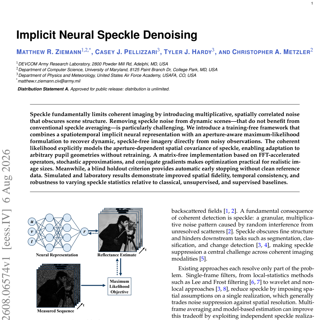
The load-bearing object is the aperture-aware coherent maximum-likelihood loss of Eq. (4), whose per-frame covariance $\Sigma_t = A D(r_t) A^H + \sigma^2 I$ encodes how the pupil $p$ broadens the point-spread function and correlates speckle across pixels. A spatiotemporal WIRE network (a wavelet implicit neural representation, a multilayer perceptron with complex Gabor activations) serves as the reflectance prior, mapping coordinates $(u,v,t)$ to nonnegative reflectance, with a tuned low oscillation frequency that favors low-frequency scene structure early in fitting. The loss is evaluated matrix-free: FFTs apply the covariance, stochastic Lanczos quadrature estimates the log-determinant, and conjugate gradients solve the inverse quadratic form, giving per-frame cost $O((SK+G)N\log N)$. A blind holdout rule stops optimization at the minimum of the held-out likelihood.

What would settle it

A deciding test is to simulate a sequence in which the complex speckle field is correlated across time (so $g_t$ changes smoothly rather than independently between frames) while keeping the same pupil, then run the method with blind holdout stopping and compare the stop point against the oracle-MSE minimum; if the holdout likelihood stops far from the true optimum or the recovered reflectance falls below an aperture-matched supervised baseline, the independence assumption in the likelihood is the failure point.

Watch

Extended reading notes

Core claim

The central discovery is that the covariance structure of fully developed speckle, written as $\Sigma_t = A D(r_t) A^H + \sigma^2 I$ with $A = F^H D(p) F$ the coherent propagation operator through pupil $p$, turns denoising into a tractable maximum-likelihood problem when combined with an implicit neural representation. The paper argues that optimizing the network parameters $\theta$ against this likelihood, instead of a generic pixelwise loss, is what lets the reconstruction separate shared scene reflectance from frame-specific speckle, and that the same likelihood evaluated on two held-out frames provides a reference-free early-stopping signal. The method is training-free in the sense that each sequence is denoised by a fresh optimization, and aperture changes are handled by the pupil mask in the forward model rather than by retraining.

Load-bearing premise

The method assumes the scene is a matte, rough reflector whose speckle noise is independent from pixel to pixel and from frame to frame, and that the optical path adds no time-varying phase errors; if those conditions fail, the covariance model the loss is built on no longer describes the measurements.

Editorial extensions

If this is right

A single noisy measurement sequence, plus knowledge of the pupil, is enough to denoise dynamic coherent imagery; no clean reference frames, external datasets, motion estimates, or aperture-specific retraining are needed.
The same objective transfers to different pupil geometries—large, small, annular, and sparse Golay apertures—by changing only the pupil mask $p$, so a new sensor geometry does not require collecting matched training data.
Blind holdout early stopping makes the per-sequence optimization fully automatic, removing model selection as a practical barrier.
On simulated DERF-HD videos the method reports the best PSNR, SSIM, and ST-RRED among compared methods for large and small apertures, and on laboratory digital holography it preserves fine resolution-bar structure and temporal stability.
The matrix-free likelihood evaluation scales from explicit-covariance infeasibility at $256\times 256$ to practical operation at $512\times 512$, with per-frame denoising runtimes near 85 seconds at $256\times 256$.

Reading between the lines

Editorial extensions of the paper, not claims the author makes directly.

Because the holdout MLE is claimed to track the unobservable oracle MSE, the same stopping rule could plausibly transfer to other inverse problems with known forward covariances, such as multi-look digital holography or partial-coherence tomography; the paper does not test this transfer.
A natural extension the paper leaves implicit is joint estimation of the pupil or static aberrations along with reflectance, since the likelihood already depends on $p$; if the pupil is only approximately known, the method's advantage over retrained baselines may shrink.
The reported improvement with temporal window length up to 32 frames suggests that adaptive windowing or larger INR capacity could push performance further on longer sequences, but the paper fixes window size and architecture.
The matrix-free approximations (stochastic Lanczos quadrature and conjugate gradients) introduce a small PSNR loss relative to the explicit likelihood; replacing them with cheaper deterministic estimators could reduce runtime further, though the paper does not explore that direction.

Share X Bluesky LinkedIn Reddit HN

Signed reviews

No signed human review yet.

Editorial analysis

A structured set of objections, weighed in public.

Desk editor's note, referee report, and a circularity audit.

Desk Editor's Note

read the letter

Short version: this is a real advance and deserves refereeing. The method—fitting a spatiotemporal INR to a coherent MLE loss that models aperture-induced speckle covariance, with a matrix-free implementation and a blind holdout stopping rule—is new as a package, and the validation is mostly honest. But the headline numbers are produced under the model's own temporal-independence assumption, and the only physical moving-target evidence is qualitative. Don't take Table 2 as proof that the gains survive for speckle that translates with the scene.

What's good: the likelihood is derived from standard Goodman speckle physics, not reverse-engineered from the results. The matrix-free trick (FFT covariance + SLQ + CG) is legit and validated against explicit evaluation (PSNR 22.4 vs 22.0; SSIM 0.71 vs 0.69). The ablations show that both the tuned WIRE backbone and the MLE loss matter: replacing MLE with intensity MSE drops PSNR from 27.9 to 25.7, and using the original WIRE hyperparameters drops it to 23.7. The baselines are strong, including aperture-retrained supervised models, and DVP is given oracle early stopping. The lab experiments with a real holography setup, including a pupil change to an annular aperture, are convincing evidence that the method is not purely a simulation artifact.

Soft spots. The big one: Eq. (4) assumes independent speckle and noise realizations across time. For a rigidly translating rough object, the complex reflectivity is a fixed random field; the speckle pattern translates and is correlated frame-to-frame. The simulated data generation draws a fresh g_t per frame, so Table 2 validates the algorithm under exactly the assumption of the likelihood. That's a clean in-model demonstration, but it does not test the physical moving-target scenario. The lab experiments use translating targets and do show qualitative improvement, which is reassuring, but there are no quantitative metrics. The authors acknowledge temporal speckle correlation in Section 4, but it sits right on the main claim. I'd ask them to add a simulation where the speckle field is a single fixed random draw shifted per frame (with and without additive noise) and see how much the margin shrinks. That would either shore up the claim or bound it honestly.

Minor issues: the noise variance sigma for the lab likelihood is never stated, which makes the lab results hard to reproduce. Table 2 reports averages without error bars across the seven DERF-HD sequences. No code or data is released (the data availability note says 'not publicly available at this time'), which for a methods-heavy paper is a real cost. The early-stopping patience is set separately for simulated (150) and lab (750) data; there is no sensitivity analysis. All fixable.

Who's it for: computational imaging researchers working on SAR, digital holography, or OCT. I'd send it to a strong referee. It's not a desk reject. The core physics is right; the soft spots are about verification breadth and documentation, not a wrong derivation.

Referee Report

2 major / 4 minor

Summary. The paper proposes a training-free framework for denoising dynamic coherent imagery by fitting a spatiotemporal implicit neural representation (INR) to noisy complex-field measurements with an aperture-aware maximum-likelihood objective. The likelihood models the measurement covariance as Sigma_t = A D(r_t) A^H + sigma^2 I, where A encodes pupil propagation, and is made practical through FFT-based covariance products, stochastic Lanczos quadrature for the log-determinant, and conjugate gradients for the quadratic form. A blind holdout criterion using two withheld frames provides early stopping without clean references. Experiments on simulated DERF-HD videos under large, small, and Golay apertures report improvements in PSNR, SSIM, and ST-RRED over classical (H-BM3D), unsupervised (DVP), and supervised (DRUNet, FastDVDNet) baselines, including aperture-retrained variants. Laboratory off-axis holography experiments with translating targets and circular and annular apertures show qualitative improvements in spatial detail and temporal consistency.

Significance. If the results hold, the work is significant: it couples coherent-imaging physics to INR priors, requires no external clean training data, adapts to known pupil geometries without retraining, and provides a matrix-free implementation that scales to realistic resolutions. The blind holdout stopping rule is a practical contribution, and the comparison against aperture-retrained supervised baselines is unusually thorough. However, the central dynamic-scene claim is weakened by the temporal-independence assumption in the likelihood: the quantitative simulated validation is performed under the model's own assumption of independent speckle per frame, while the physically motivated dynamic-scene regime involves temporally correlated speckle for translating rough objects.

major comments (2)

[Section 2A, Eq. (4); Supplement 4; Section 4] The sequence-level likelihood in Eq. (4) is derived under independent speckle and additive-noise realizations over time, and the simulated measurements are generated with a fresh g_t for each frame, so Table 2 validates the method under exactly this independence assumption. For a rigidly translating rough object, the object-plane complex field is a single fixed random field shifted across frames, so the image-plane speckle is strongly correlated in time and Eq. (4) is a composite likelihood rather than the joint likelihood. This assumption is load-bearing for the paper's central dynamic-scene claim: the reported PSNR/SSIM/ST-RRED margins may rely on temporal averaging of independent speckle. Section 4 lists temporal speckle correlation as a limitation, but that is precisely the regime the title and introduction target. The laboratory translating-target experiments provide genuine qualitative evidence of robustness, but they do not quantify the margins under correlated speckle. Please add simulated experiments with physically correlated speckle (for example, a fixed complex reflectivity translated by a known motion between frames) and report the same metrics, or temper the dynamic-scene claim accordingly.
[Supplement 1, Fig. S1] The validation of the matrix-free approximation reports PSNR 22.4 versus 22.0 dB and SSIM 0.71 versus 0.69, but ST-RRED degrades from 13,486 to 22,945, roughly a 70% increase. Since all main results use the matrix-free implementation and Table 2 reports ST-RRED as a headline temporal-consistency metric, the approximation error in ST-RRED should be characterized at the resolution and aperture conditions used in Table 2, or the reported ST-RRED values should be interpreted with this caveat. The current explanation attributes the discrepancy to low resolution and metric sensitivity, but it does not establish that the effect is negligible at 256x256.

minor comments (4)

[Section 2C and Supplement 1, Section 3] The main text should state explicitly that the two withheld frames are included in the PSNR, SSIM, and ST-RRED evaluations; this disclosure currently appears only in the supplement.
[Section 3C, Table 3] The ablation study is performed on a single DERF-HD sequence (sunflower); including a second sequence would increase confidence that the conclusions about architecture and loss are not sequence-specific.
[Section 1] The phrase 'training-free' should be clarified to mean no external training data or pretrained weights, since the INR is still optimized per sequence; the current wording could be misread as claiming no optimization at all.
[Section 3B, Golay aperture paragraph] The text states that 'our method continues to outperform all baselines' for the Golay aperture, but the following sentence reports that PSNR matches FastDVDNet-A at 22.2 dB; please qualify the claim by noting that the improvement is in SSIM and ST-RRED rather than PSNR.

Circularity Check

0 steps flagged · score 0.0 of 10

No significant circularity: the coherent likelihood comes from external speckle physics, the INR is a generic prior, and the blind holdout criterion is evaluated on withheld frames; the only caveats are model-misspecification and validation selection, not circular derivation.

full rationale

The derivation chain is self-contained rather than circular. Equation (4) follows from the fully developed speckle model g_t ~ CN(0,I), the linear pupil propagation A = F^H D(p) F, and additive noise, all from Goodman's external speckle statistics; the target reflectance r_t is the unknown parameter of this likelihood, not a quantity presupposed by it. The INR is a standard WIRE coordinate network whose hyperparameters (omega0=1, s0=2) are disclosed and ablated against SIREN, MLP, original WIRE, and MSE loss (Table 3), so no ansatz is smuggled via citation. Blind holdout early stopping evaluates the MLE loss on frames 12 and 28, which are withheld from the optimization loss; the network is not fit to those measurements, so the stopping signal is not a re-statement of the training loss. One minor protocol caveat is that the two held-out frames used for early stopping are also included in the reported metrics, which can slightly favor the chosen checkpoint, but this does not make the predicted reflectance equal to the fitted loss or to the input measurements. The simulated experiments generate data from the same forward model, which is a within-model consistency check rather than independent physical validation; this is a limitation, not a circularity. The laboratory digital holography experiments provide real-data evidence, and Section 4 explicitly acknowledges the fully developed speckle and temporal-independence assumptions and the need for richer object models, an honest limitation statement rather than a hidden circular step. The only self-citations (the preliminary SPIE paper [38] and co-authored demodulation/imaging references) are acknowledgments or implementation details, not load-bearing evidence for the central claim; no uniqueness theorem or ansatz is imported from the authors' prior work. Therefore no step reduces to its own inputs by construction.

Assumptions & free parameters 8 free parameters · 5 assumptions · 0 invented entities

The central claim rests on the standard fully developed speckle model, a static-pupil propagation model, temporal independence, the known Gaussian measurement-noise model, and the empirical assumption that a tuned WIRE network provides a suitable prior for dynamic reflectance. The algorithm also depends on hand-tuned hyperparameters (omega0, s0, patience, window length, solver settings). No new physical entities are introduced. The least documented input is sigma for the laboratory data.

free parameters (8)

WIRE oscillation frequency omega0 = 1.0
Set lower than the published WIRE variant to bias fitting toward low frequencies; tuned on simulated speckle sequences and affects all reported results (Sec. 2B).
WIRE Gaussian envelope width s0 = 2.0
Set lower than the published WIRE variant to encourage smoother frequency transitions; tuned jointly with omega0 (Sec. 2B).
Early stopping patience = 150 (simulation), 750 (lab)
Patience thresholds for the blind holdout criterion, selected per dataset; lab value increased to avoid premature stopping on sparse low-frequency bar targets (Supplement 3).
Holdout loss smoothing window = 15 iterations (lab only)
Temporal smoothing applied to the lab holdout loss to reduce noise in the stopping signal (Supplement 3).
Temporal window length = 32 frames
Selected based on Table S1 tradeoff: performance improves from 4 to 32 frames and saturates at 64; used throughout the paper (Supplement 8).
SLQ/CG solver settings = S=8 probes, K=20 Lanczos iterations, G=200 CG iterations
Fixed approximation parameters chosen for practical accuracy/cost; validated against explicit MLE at 64x64 (Supplement 2).
Noise level sigma = 0.02 (simulation); lab value unspecified
Simulation uses sigma=0.02 (Sec. 3B); the lab experiments do not state how sigma is set or estimated, yet the likelihood Eq. (4) requires it.
INR architecture capacity = 12 hidden layers, 362 complex neurons per layer (1.6M parameters)
Fixed model capacity chosen for the experiments; the paper notes larger windows may need wider or deeper networks (Sec. 2B).

assumptions (5)

domain assumption Fully developed speckle: object-plane field is r_t^{1/2} o g_t with g_t ~ CN(0, I), independent across pixels and time (Eq. 2).
Standard Goodman model for rough diffuse scatterers; the reflectance r_t is identified with the per-pixel variance of the speckle field.
domain assumption Coherent propagation through a sampled pupil with real-valued transmission p and negligible time-varying phase errors (Eq. 1).
A = F^H D(p) F assumes an isoplanatic, static pupil; lab data are corrected for static aberrations but time-varying errors are excluded.
domain assumption Temporal independence of speckle and additive noise realizations across frames (Sec. 2A).
Required to factor the sequence likelihood into per-frame terms in Eq. (4); valid when object motion fully decorrelates speckle between frames.
domain assumption The WIRE INR with 12 layers of 362 complex neurons and low omega0/s0 provides an appropriate implicit prior for dynamic reflectance sequences.
Relies on the spectral bias of INRs to fit low-frequency scene structure before noise; validated empirically (Table 3) but not proven.
domain assumption Additive measurement noise is circular complex Gaussian n_t ~ CN(0, sigma^2 I) with known sigma^2.
Standard sensor noise model; sigma^2 is an input to the likelihood and is specified for simulation but unspecified for lab data.

how reviews work

0 comments

Cite this review

Pith. "Pith review of Implicit Neural Speckle Denoising." pith.science (2026). https://pith.science/paper/B5CWDL4N

@misc{pith2026260806574,
  author       = {Pith},
  title        = {Pith review of: Implicit Neural Speckle Denoising},
  year         = {2026},
  howpublished = {\url{https://pith.science/paper/B5CWDL4N}},
  note         = {Machine review of arXiv:2608.06574}
}

read the original abstract

Speckle fundamentally limits coherent imaging by introducing multiplicative, spatially correlated noise that obscures scene structure. Removing speckle noise from dynamic scenes--that do not benefit from conventional speckle averaging--is particularly challenging. We introduce a training-free framework that combines a spatiotemporal implicit neural representation with an aperture-aware maximum-likelihood formulation to recover dynamic, speckle-free imagery directly from noisy observations. The coherent likelihood explicitly models the aperture-dependent spatial covariance of speckle, enabling adaptation to arbitrary pupil geometries without retraining. A matrix-free implementation based on FFT-accelerated operators, stochastic approximations, and conjugate gradients makes optimization practical for realistic image sizes. Meanwhile, a blind holdout criterion provides automatic early stopping without clean reference data. Simulated and laboratory results demonstrate improved spatial fidelity, temporal consistency, and robustness to varying speckle statistics relative to classical, unsupervised, and supervised baselines.

Figures

Figures reproduced from arXiv: 2608.06574 by the authors.

**Figure 1.** Implicit neural speckle denoising. A spatiotemporal INR is optimized directly from noisy coherent measurements using an aperture-aware maximumlikelihood objective, enabling dynamic speckle denoising without prior training. 1. INTRODUCTION Coherent imaging systems—including synthetic aperture radar (SAR), digital holography, and optical coherence tomography—measure the amplitude and phase of backscattered fields… view at source ↗

**Figure 2.** Spatially correlated speckle. Simulated coherent measurements generated using large (left) and small (right) aperture sizes at fixed sensor-plane sampling. Smaller relative apertures produce larger speckle grains and stronger spatial correlations, making denoising more challenging. Insets show the aperture in white and sampled frequency support in red. model coherent propagation through the sampled pupil as A = F HD… view at source ↗

**Figure 3.** Denoising neural architecture. Diagram of the modified wavelet implicit neural representation (WIRE [27]) used to optimize the likelihood-based loss for denoising. coherent propagation. Since minimizing this objective yields the maximum-likelihood estimate of the reflectance parameters, we refer to it as the MLE loss throughout the paper. A full likelihood derivation is provided in Supplement 1. B. Spatiotemporal i… view at source ↗

Figures from the paper (5 more)

**Figure 5.** Figure 5: Temporally consistent denoising. Simulated small-aperture speckle denoising on translating cameraman (left) and DERF-HD tractor (right) sequences. The x–t plots stack intensities along the indicated horizontal line across time. Our method recovers greater detail with m…

**Figure 6.** Figure 6: Aperture-aware denoising. Simulated Golay-aperture speckle denoising on translating cameraman (left) and DERF-HD tractor (right) sequences. Our method recovers greater detail with more stable temporal trajectories. Supplemental videos more clearly illustrate denoising…

**Figure 7.** Figure 7: Laboratory data collection. Off-axis digital holography setup used to collect speckled videos of moving objects. A signal path flood-illuminates targets 2.6 m away, and the return interferes with a fiber-delivered reference beam at the camera. Measurement DRUNet-A Fast…

**Figure 8.** Figure 8: Improved detail recovery on laboratory data. Intensity profiles across laboratory USAF resolution bars. Our method preserves more distinct peaks and valleys, indicating improved recovery of fine spatial structure. the translating object without sudden frame-to-frame va…

**Figure 9.** Figure 9: Temporally consistent laboratory denoising. Digital holography denoising of a translating toy target measured with a conventional circular aperture (left) and a translating resolution target measured with an annular aperture (right). Our method retains more temporall…

Review history (2 revisions) →

Discussion (0). Continue with ORCID to comment.

Reference graph

Works this paper leans on

21 extracted references · 20 canonical work pages

[1]

Multilook Coherent Imaging: Theoretical Guarantees and Algorithms

X. Chen, S. Jana, C. A. Metzler,et al., “Multilook coherent imaging: Theoretical guarantees and algorithms,” arXiv preprint arXiv:2505.23594 (2025)

work page Pith review arXiv 2025
[2]

Fast estimation oftr(f(a)) via stochastic lanczos quadrature,

S. Ubaru, J. Chen, and Y. Saad, “Fast estimation oftr(f(a)) via stochastic lanczos quadrature,” SIAM J. Matrix Anal. Appl.38, 1075–1099 (2017)

work page 2017
[3]

Scalable log determinants for gaussian process kernel learning,

K. Dong, D. Eriksson, H. Nickisch,et al., “Scalable log determinants for gaussian process kernel learning,” inAdvances in Neural Information Processing Systems,vol. 30 I. Guyon, U. V . Luxburg, S. Bengio,et al., eds. (Curran Associates, Inc., 2017)

work page 2017
[4]

A stochastic estimator of the trace of the influence matrix for laplacian smoothing splines,

M. Hutchinson, “A stochastic estimator of the trace of the influence matrix for laplacian smoothing splines,” Commun. Stat. - Simul. Comput.18, 1059–1076 (1989)

work page 1989
[5]

Methods of conjugate gradients for solving linear systems,

M. R. Hestenes and E. Stiefel, “Methods of conjugate gradients for solving linear systems,” J. research National Bureau Stand.49, 409–436 (1952)

work page 1952
[6]

PyTorch: An imperative style, high-performance deep learning library,

A. Paszke, S. Gross, F. Massa,et al., “PyTorch: An imperative style, high-performance deep learning library,” Adv. Neural Inf. Process. Syst.32(2019)

work page 2019
[7]

Image denoising by sparse 3-D transform- domain collaborative filtering,

K. Dabov, A. Foi, V . Katkovnik, and K. Egiazarian, “Image denoising by sparse 3-D transform- domain collaborative filtering,” IEEE Trans. Image Process.16, 2080–2095 (2007)

work page 2007
[8]

MuLoG, or how to apply gaussian denoisers to multi-channel SAR speckle reduction?

C.-A. Deledalle, L. Denis, S. Tabti, and F. Tupin, “MuLoG, or how to apply gaussian denoisers to multi-channel SAR speckle reduction?” IEEE Trans. Image Process.26, 4389–4403 (2017)

work page 2017

Show all 21 references

[9]

Deep video prior for video consistency and propagation,

C. Lei, Y. Xing, H. Ouyang, and Q. Chen, “Deep video prior for video consistency and propagation,” IEEE Trans. Pattern Anal. Mach. Intell.45, 356–371 (2023)

2023
[10]

Plug-and-play image restoration with deep denoiser prior,

K. Zhang, Y. Li, W. Zuo,et al., “Plug-and-play image restoration with deep denoiser prior,” IEEE Trans. Pattern Anal. Mach. Intell.44, 6360–6376 (2022)

2022
[11]

NTIRE 2017 challenge on single image super-resolution: Dataset and study,

E. Agustsson and R. Timofte, “NTIRE 2017 challenge on single image super-resolution: Dataset and study,” inThe IEEE Conference on Computer Vision and Pattern Recognition (CVPR) Workshops,(2017)

2017
[12]

Fastdvdnet: Towards real-time deep video denoising without flow estimation,

M. Tassano, J. Delon, and T. Veit, “Fastdvdnet: Towards real-time deep video denoising without flow estimation,” inProceedings of the IEEE/CVF conference on computer vision and pattern recognition,(2020), pp. 1354–1363

2020
[13]

The 2017 DAVIS challenge on video object segmen- tation,

J. Pont-Tuset, F. Perazzi, S. Caelles,et al., “The 2017 DAVIS challenge on video object segmen- tation,” arXiv preprint arXiv:1704.00675 (2017)

2017 arXiv
[14]

Image quality assessment: from error visibility to structural similarity,

Z. Wang, A. C. Bovik, H. R. Sheikh, and E. P . Simoncelli, “Image quality assessment: from error visibility to structural similarity,” IEEE Trans. Image Process.13, 600–612 (2004)

2004
[15]

Video quality assessment by reduced reference spatio- temporal entropic differencing,

R. Soundararajan and A. C. Bovik, “Video quality assessment by reduced reference spatio- temporal entropic differencing,” IEEE Trans. Circuits Syst. Video Technol.23, 684–694 (2013)

2013
[16]

A comparison of patch-based models in video denoising,

P . Arias, G. Facciolo, and J.-M. Morel, “A comparison of patch-based models in video denoising,” in2018 IEEE 13th Image, Video, and Multidimensional Signal Processing Workshop 8 (IVMSP),(2018), pp. 1–5

2018
[17]

Xiph.org Video Test Media [derf’s collection],

Xiph.org Foundation, “Xiph.org Video Test Media [derf’s collection],”https://media.xiph.org/ video/derf/
[18]

A golay metalens for long-range, large aperture, thermal imaging via sparse aperture computational imaging,

J. Wang, A. Wirth-Singh, V . Saragadam,et al., “A golay metalens for long-range, large aperture, thermal imaging via sparse aperture computational imaging,” Nat. Commun.16, 10281 (2025)

2025
[19]

Deep-turbulence wavefront sensing using digital-holographic detection in the off-axis image plane recording geometry,

M. F. Spencer, R. A. Raynor, M. T. Banet, and D. K. Marker, “Deep-turbulence wavefront sensing using digital-holographic detection in the off-axis image plane recording geometry,” Opt. Eng.56, 031213–031213 (2017)

2017
[20]

Phase-error estimation and image recon- struction from digital-holography data using a bayesian framework,

C. J. Pellizzari, M. F. Spencer, and C. A. Bouman, “Phase-error estimation and image recon- struction from digital-holography data using a bayesian framework,” J. Opt. Soc. Am. A Opt. Image Sci. Vis.34, 1659–1669 (2017)

2017
[21]

Phase-error correction in digital holography using single-shot data,

S. T. Thurman, “Phase-error correction in digital holography using single-shot data,” JOSA A36, D47–D61 (2019). 9

2019

Pith tools

Reviewed August 15, 2026 · model on record in the stance chip above.

[1] [1]

Multilook Coherent Imaging: Theoretical Guarantees and Algorithms

X. Chen, S. Jana, C. A. Metzler,et al., “Multilook coherent imaging: Theoretical guarantees and algorithms,” arXiv preprint arXiv:2505.23594 (2025)

work page Pith review arXiv 2025

[2] [2]

Fast estimation oftr(f(a)) via stochastic lanczos quadrature,

S. Ubaru, J. Chen, and Y. Saad, “Fast estimation oftr(f(a)) via stochastic lanczos quadrature,” SIAM J. Matrix Anal. Appl.38, 1075–1099 (2017)

work page 2017

[3] [3]

Scalable log determinants for gaussian process kernel learning,

K. Dong, D. Eriksson, H. Nickisch,et al., “Scalable log determinants for gaussian process kernel learning,” inAdvances in Neural Information Processing Systems,vol. 30 I. Guyon, U. V . Luxburg, S. Bengio,et al., eds. (Curran Associates, Inc., 2017)

work page 2017

[4] [4]

A stochastic estimator of the trace of the influence matrix for laplacian smoothing splines,

M. Hutchinson, “A stochastic estimator of the trace of the influence matrix for laplacian smoothing splines,” Commun. Stat. - Simul. Comput.18, 1059–1076 (1989)

work page 1989

[5] [5]

Methods of conjugate gradients for solving linear systems,

M. R. Hestenes and E. Stiefel, “Methods of conjugate gradients for solving linear systems,” J. research National Bureau Stand.49, 409–436 (1952)

work page 1952

[6] [6]

PyTorch: An imperative style, high-performance deep learning library,

A. Paszke, S. Gross, F. Massa,et al., “PyTorch: An imperative style, high-performance deep learning library,” Adv. Neural Inf. Process. Syst.32(2019)

work page 2019

[7] [7]

Image denoising by sparse 3-D transform- domain collaborative filtering,

K. Dabov, A. Foi, V . Katkovnik, and K. Egiazarian, “Image denoising by sparse 3-D transform- domain collaborative filtering,” IEEE Trans. Image Process.16, 2080–2095 (2007)

work page 2007

[8] [8]

MuLoG, or how to apply gaussian denoisers to multi-channel SAR speckle reduction?

C.-A. Deledalle, L. Denis, S. Tabti, and F. Tupin, “MuLoG, or how to apply gaussian denoisers to multi-channel SAR speckle reduction?” IEEE Trans. Image Process.26, 4389–4403 (2017)

work page 2017